
 chart
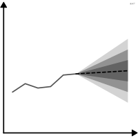
fan chart
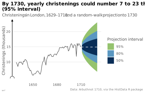
Forecast surrounded by widening uncertainty bands.
Classification
- chart
- lines and areas › areas
- change over time; Financial Times Visual Vocabulary
- the name evokes: object
Channels
 position on common scale; main: central forecast
 length; secondary: width of the interval
 color luminance; main: probability level (increasingly lighter bands)
 color saturation; main: probability level (instead of luminance)
Scientific literature
OpenAlex: 294 papers since 1999, 22% in the last five years; mostly in Economics, Econometrics and Finance, Decision Sciences, Physics and Astronomy
Seminal references
- invention (1996) Bank of England (1996). Inflation Report, February
- formalization (1998) Britton, Fisher & Whitley (1998). The Inflation Report projections: understanding the fan chart. Bank of England Quarterly Bulletin
R packages
- R
fanplot::fan(); GitHub 7 stars; last commit 2026-01
R code of the ggplot2 example
library(ggplot2)
library(dplyr)
library(HistData)
library(forecast)
## Yearly christenings in London, 1629-1710, projected 20 years ahead.
## auto.arima settles on a random walk: a flat projection, whose
## uncertainty grows with the square root of the horizon.
christenings <- ts(Arbuthnot$Total, start = 1629)
f <- forecast(auto.arima(christenings), h = 20, level = c(50, 80, 95))
bands <- bind_rows(lapply(seq_along(f$level), function(i) {
tibble(year = as.numeric(time(f$mean)), low = f$lower[, i], high = f$upper[, i],
level = paste0(f$level[i], "%"))
})) |>
mutate(level = factor(level, levels = c("95%", "80%", "50%"), ordered = TRUE))
observed <- tibble(year = Arbuthnot$Year, total = Arbuthnot$Total)
projected <- tibble(year = c(1710, as.numeric(time(f$mean))),
total = c(tail(Arbuthnot$Total, 1), as.numeric(f$mean)))
p <- ggplot() +
geom_ribbon(data = bands, aes(x = year, ymin = low, ymax = high, fill = level)) +
geom_line(data = observed, aes(x = year, y = total), colour = "#535353", linewidth = 0.5) +
geom_line(data = projected, aes(x = year, y = total), colour = "white", linewidth = 0.5,
linetype = "dashed") +
scale_fill_ordinal(type = idest_seq[c(2, 4, 6)], name = "Projection interval") +
scale_y_continuous(labels = lex_number, breaks = lex_break_breaks, expand = lex_break_expand) +
labs(title = "By 1730, yearly christenings could number 7 to 23 thousand\n(95% interval)",
subtitle = "Christenings in London, 1629–1710, and a random-walk projection to 1730",
x = NULL, y = "Christenings (thousands)",
caption = "Data: Arbuthnot 1710, via the HistData R package") +
theme_lex_viz(grid = "y", arrows = "y", break_not_zero = "y") +
theme(legend.position = "right")Sources (9)
12 occurrences in the corpus; indexed by 2 books
- app.flourish.studio
- Better data visualizations: a guide for scholars, researchers, and wonks
- Data Viz Project
- datavizproject.com
- Information Graphics: A Comprehensive Illustrated Reference
- The book of circles: visualizing spheres of knowledge
- The book of trees: visualizing branches of knowledge
- The Truthful Art: Data, Charts, and Maps for Communication
- Wikipedia in English↗
Cite this entry
Stable addresshttps://dataviz.adrientaudiere.com/en-only/term/fan-chart.html
ReferenceTaudière Adrien. 2026. fan chart. In Visualization Vocabulary, version 1.0.0. IdEst. https://dataviz.adrientaudiere.com/en-only/term/fan-chart.html
BibTeX
@incollection{taudiere2026-fan-chart,
  author    = {Taudière, Adrien},
  title     = {fan chart},
  booktitle = {Visualization Vocabulary},
  year      = {2026},
  version   = {1.0.0},
  publisher = {IdEst},
  url       = {https://dataviz.adrientaudiere.com/en-only/term/fan-chart.html},
  note      = {CC0 1.0}
}Page created on 2026-10-13. Text last changed on 2026-11-02. Images last changed on 2026-11-12. Numbers computed on 2026-10-22.