
 chart
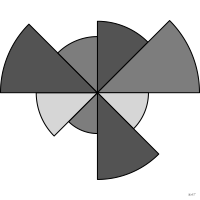
polar area chart
also: rose chart, coxcombEqual-angle sectors whose radius encodes the value.
Classification
- chart
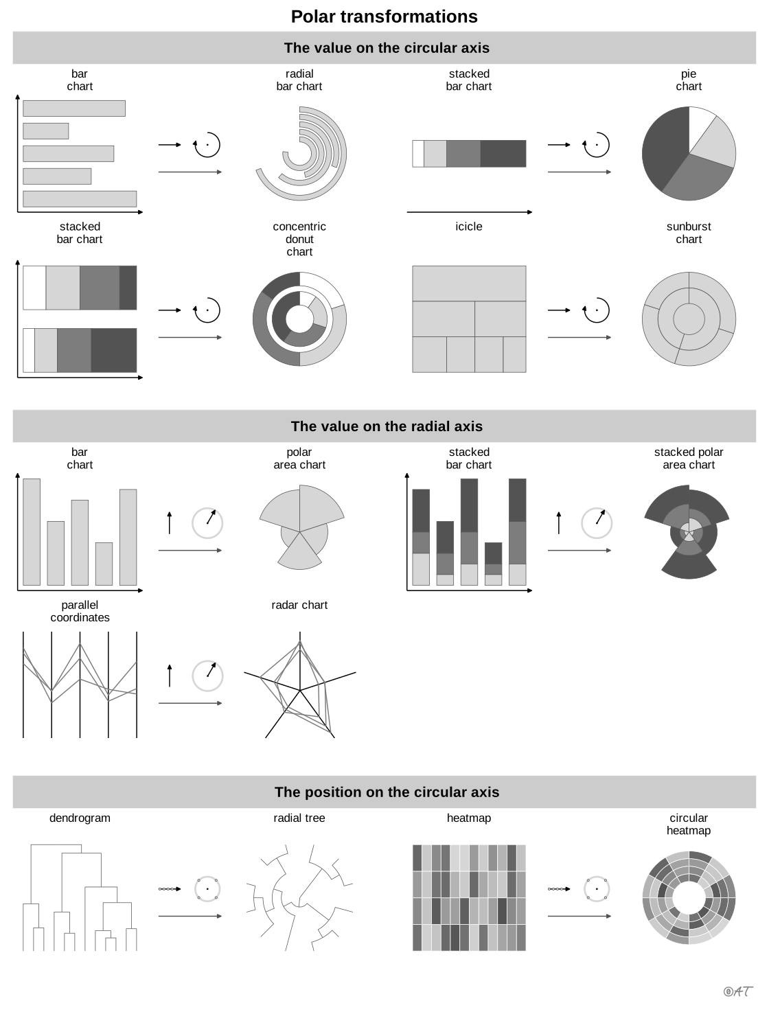
- radial › polar bars
- magnitude, part-to-whole
- the name evokes: nature
Channels
 length; main: value (sector radius (Munzner)); Munzner 2014
 area; secondary: value (perceived through area, which grows as the square of the radius); Munzner 2014
 spatial region; main: category (one sector per category); Munzner 2014
Variants
 wind rosespecial case
Scientific literature
OpenAlex: 35 papers since 2011, 40% in the last five years; mostly in Energy, Arts and Humanities, Computer Science
Seminal references
- first known use (1829) Balbi & Guerry (1829). Tableau des variations météorologiques comparées aux phénomènes physiologiques. Annales d'hygiène publique et de médecine légale; Friendly & Denis 2001, Andrews 2017
- diffusion (1857) Nightingale (1857). Mortality of the British Army. Harrison and Sons; Friendly & Denis 2001
R packages
- R
ggplot2::coord_polar(); GitHub 7 025 stars; last commit 2026-10; paper (33 455 citations)
R code of the ggplot2 example
library(ggplot2)
library(dplyr)
library(tidyr)
library(HistData)
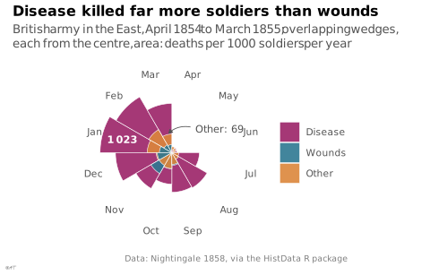
## Nightingale's first year, April 1854 to March 1855. The wedges overlap, as
## in her diagram: the largest is drawn first, so that none hides another.
year1 <- Nightingale |>
filter(Date < as.Date("1855-04-01")) |>
mutate(Month = factor(as.character(Month), levels = unique(as.character(Month)))) |>
select(Month, Disease = Disease.rate, Wounds = Wounds.rate, Other = Other.rate) |>
pivot_longer(-Month, names_to = "cause", values_to = "rate") |>
mutate(cause = factor(cause, levels = c("Disease", "Wounds", "Other"))) |>
arrange(desc(rate)) |>
mutate(order = row_number())
## Two values read out: disease in January, other causes in March.
jan <- year1$rate[year1$Month == "Jan" & year1$cause == "Disease"]
mar <- year1$rate[year1$Month == "Mar" & year1$cause == "Other"]
## A square-root scale makes the area of each wedge, not its radius,
## proportional to the rate, as Nightingale drew it.
## Months as numbers (April = 1, March = 12) so the March label can sit in the
## empty April-June wedges: past 12.5 the angle wraps round to April, and the
## arrow crosses the March/April boundary instead of circling the whole chart.
months <- levels(year1$Month)
p <- ggplot(year1, aes(x = as.integer(Month), y = rate, fill = cause, group = order)) +
geom_col(width = 1, position = "identity", colour = "white", linewidth = 0.2, alpha = 0.9) +
annotate("text", x = 10, y = jan / 2, label = lex_number(round(jan)), size = 3,
colour = "white", fontface = "bold") +
annotate("segment", x = 13.7, xend = 12.2, y = 200, yend = mar + 8, colour = "#535353",
linewidth = 0.3, arrow = grid::arrow(length = unit(1.2, "mm"), type = "closed")) +
annotate("text", x = 14, y = 220, label = paste("Other:", round(mar)), hjust = 0, size = 3,
colour = "#535353") +
coord_polar() +
scale_x_continuous(limits = c(0.5, 12.5), breaks = 1:12, labels = months, oob = scales::oob_keep) +
scale_y_sqrt(breaks = NULL) +
labs(title = "Disease killed far more soldiers than wounds",
subtitle = "British army in the East, April 1854 to March 1855; overlapping wedges, each from the centre, area: deaths per 1\u2009000 soldiers per year",
x = NULL, y = NULL, fill = NULL,
caption = "Data: Nightingale 1858, via the HistData R package") +
theme_lex_viz(grid = "", arrows = "") +
theme(legend.position = "right")Sources (17)
55 occurrences in the corpus; indexed by 6 books
Show the 17 sources
- Atlas of knowledge: anyone can map
- Better data visualizations: a guide for scholars, researchers, and wonks
- Cartographies of Time
- Data visualisation: a handbook for data driven design
- Data Viz Project
- datavizproject.com
- Design for information: an introduction to the histories, theories, and best practices ...
- Effective data storytelling: how to drive change with data, narrative, and visuals
- Friendly & Wainer, A History of Data Visualization and Graphic Communication, Harvard University Press, 2021
- Information Graphics: A Comprehensive Illustrated Reference
- Interactive data visualization: foundations, techniques, and applications
- Milestones in the history of thematic cartography, statistical graphics, and data visua...
- Questions in Dataviz: A Design-Driven Process for Data Visualisation
- The book of circles: visualizing spheres of knowledge
- The grammar of graphics
- Visualization Analysis and Design
- Visualization of Time-Oriented Data
Cite this entry
Stable addresshttps://dataviz.adrientaudiere.com/en-only/term/polar-area-chart.html
ReferenceTaudière Adrien. 2026. polar area chart. In Visualization Vocabulary, version 1.0.0. IdEst. https://dataviz.adrientaudiere.com/en-only/term/polar-area-chart.html
BibTeX
@incollection{taudiere2026-polar-area-chart,
  author    = {Taudière, Adrien},
  title     = {polar area chart},
  booktitle = {Visualization Vocabulary},
  year      = {2026},
  version   = {1.0.0},
  publisher = {IdEst},
  url       = {https://dataviz.adrientaudiere.com/en-only/term/polar-area-chart.html},
  note      = {CC0 1.0}
}Page created on 2026-10-13. Text last changed on 2026-11-02. Images last changed on 2026-11-12. Numbers computed on 2026-10-22.