
 chart
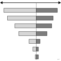
tornado chart
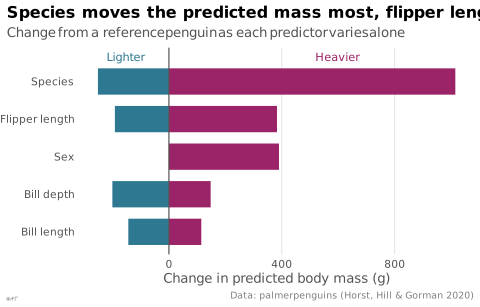
Opposed bars ranked by magnitude for a sensitivity analysis.
Classification
- chart
- bars › diverging bars
- deviation
- the name evokes: nature
Channels
 position on common scale; main: low and high value
 length; main: effect on the output
 spatial region; main: parameter, sorted by effect
 color hue; secondary: direction of the variation
Scientific literature
OpenAlex: 113 papers since 2001, 36% in the last five years; mostly in Energy, Economics, Econometrics and Finance, Engineering; Wikidata
Seminal references
R packages
- R
tornado::tornado(); GitHub 9 stars; last commit 2024-08
R code of the ggplot2 example
library(ggplot2)
library(dplyr)
library(palmerpenguins)
## Linear model of body mass. Starting from a reference penguin (a female
## Adelie with median measures), each predictor varies alone: from the 10th
## to the 90th percentile for a measure, across its values for species and sex.
birds <- filter(penguins, !is.na(sex))
model <- lm(body_mass_g ~ bill_length_mm + bill_depth_mm + flipper_length_mm + species + sex, data = birds)
reference <- data.frame(bill_length_mm = median(birds$bill_length_mm),
bill_depth_mm = median(birds$bill_depth_mm),
flipper_length_mm = median(birds$flipper_length_mm),
species = factor("Adelie", levels = levels(birds$species)),
sex = factor("female", levels = levels(birds$sex)))
change <- function(variable, values) {
others <- reference[rep(1, length(values)), ]
others[[variable]] <- values
range(predict(model, others) - predict(model, reference))
}
swings <- bind_rows(
tibble(predictor = "Bill length", range = list(change("bill_length_mm", quantile(birds$bill_length_mm, c(0.1, 0.9))))),
tibble(predictor = "Bill depth", range = list(change("bill_depth_mm", quantile(birds$bill_depth_mm, c(0.1, 0.9))))),
tibble(predictor = "Flipper length", range = list(change("flipper_length_mm", quantile(birds$flipper_length_mm, c(0.1, 0.9))))),
tibble(predictor = "Species", range = list(change("species", levels(birds$species)))),
tibble(predictor = "Sex", range = list(change("sex", levels(birds$sex))))
) |>
mutate(low = sapply(range, min), high = sapply(range, max),
predictor = reorder(predictor, high - low))
p <- ggplot(swings, aes(y = predictor)) +
geom_rect(aes(xmin = low, xmax = 0, ymin = as.integer(predictor) - 0.35, ymax = as.integer(predictor) + 0.35),
fill = "#2e7891") +
geom_rect(aes(xmin = 0, xmax = high, ymin = as.integer(predictor) - 0.35, ymax = as.integer(predictor) + 0.35),
fill = "#9b2367") +
geom_vline(xintercept = 0, colour = "#535353", linewidth = 0.4) +
annotate("text", x = c(-150, 600), y = 5.65, label = c("Lighter", "Heavier"),
colour = c("#2e7891", "#9b2367"), size = 3) +
scale_x_continuous(labels = lex_number) +
scale_y_discrete(expand = expansion(add = c(0.6, 0.9))) +
labs(title = "Species moves the predicted mass most, flipper length next",
subtitle = "Change from a reference penguin as each predictor varies alone",
x = "Change in predicted body mass (g)", y = NULL,
caption = "Data: palmerpenguins (Horst, Hill & Gorman 2020)") +
theme_lex_viz(grid = "x", arrows = "")Sources (1)
Cite this entry
Stable addresshttps://dataviz.adrientaudiere.com/en-only/term/tornado-chart.html
ReferenceTaudière Adrien. 2026. tornado chart. In Visualization Vocabulary, version 1.0.0. IdEst. https://dataviz.adrientaudiere.com/en-only/term/tornado-chart.html
BibTeX
@incollection{taudiere2026-tornado-chart,
  author    = {Taudière, Adrien},
  title     = {tornado chart},
  booktitle = {Visualization Vocabulary},
  year      = {2026},
  version   = {1.0.0},
  publisher = {IdEst},
  url       = {https://dataviz.adrientaudiere.com/en-only/term/tornado-chart.html},
  note      = {CC0 1.0}
}Page created on 2026-10-13. Text last changed on 2026-11-11. Images last changed on 2026-11-02. Numbers computed on 2026-10-22.