
 chart
hyperbolic tree
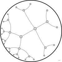
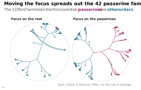
also: hypertreeNode-link tree drawn in hyperbolic geometry that enlarges the focus and squeezes the rest toward the edge of a disk.
arbre hyperbolique
Arbre nœuds-liens dessiné en géométrie hyperbolique qui agrandit le foyer et comprime le reste vers le bord du disque.
Variante de l'arbre radial (Lima) ; le foyer se déplace par translation hyperbolique (Munzner 2014).
Classification
- chart
- networks and trees › hierarchical trees
- the name evokes: nature
Channels
 spatial region; main: position in the hierarchy
 color hue; secondary: branch
Attestation
Scientific literature
OpenAlex: 101 papers since 2000, 7% in the last five years; mostly in Computer Science; Wikidata
Seminal references
- invention (1994) Lamping & Rao (1994). Laying out and visualizing large trees using a hyperbolic space. Proceedings of the 7th annual ACM symposium on User interface software and technology (UIST '94) (196 citations)
- diffusion (1995) Lamping, Rao & Pirolli (1995). A focus+context technique based on hyperbolic geometry for visualizing large hierarchies. Proceedings of the SIGCHI conference on Human factors in computing systems (CHI '95) (920 citations); The book of trees: visualizing branches of knowledge
R code of the ggplot2 example
library(ggplot2)
library(ape)
library(hydra)
## The 137 bird families of Sibley & Ahlquist in the Poincaré disk. The
## layout is hydraPlus() (Keller-Ressel & Nargang 2020): a hyperbolic
## embedding of the path lengths along the tree, which keeps the branches
## apart as they crowd toward the rim. A Möbius transformation then puts the
## focus on the root, then on the passerines, which open up while the rest
## of the tree is pushed to the edge. Links are hyperbolic geodesics: arcs
## of circles that meet the rim at right angles.
data(bird.families)
tree <- reorder(bird.families, "cladewise")
n_tip <- Ntip(tree)
tree$edge.length <- rep(1, nrow(tree$edge))
## Path lengths halved: at full length the embedding overflows (hydra warns).
embedding <- hydraPlus(dist.nodes(tree) * 0.5, dim = 2, curvature = 1,
control = list(trace = 0))
z <- complex(modulus = embedding$r, argument = embedding$theta)
passerines <- getMRCA(tree, c("Tyrannidae", "Fringillidae"))
## Cladewise order: a parent comes before its children.
in_passerines <- seq_along(z) == passerines
for (i in seq_len(nrow(tree$edge))) {
in_passerines[tree$edge[i, 2]] <- in_passerines[tree$edge[i, 2]] || in_passerines[tree$edge[i, 1]]
}
## Geodesic between p and q: a straight segment through the centre, otherwise
## the circle through p, q and the inverse of p in the unit circle.
geodesic <- function(p, q, n = 30) {
if (abs(Im(Conj(p) * q)) < 1e-9) {
return(seq(0, 1, length.out = n) * (q - p) + p)
}
r <- p / Mod(p)^2
d <- 2 * (Re(p) * (Im(q) - Im(r)) + Re(q) * (Im(r) - Im(p)) + Re(r) * (Im(p) - Im(q)))
cx <- (Mod(p)^2 * (Im(q) - Im(r)) + Mod(q)^2 * (Im(r) - Im(p)) + Mod(r)^2 * (Im(p) - Im(q))) / d
cy <- (Mod(p)^2 * (Re(r) - Re(q)) + Mod(q)^2 * (Re(p) - Re(r)) + Mod(r)^2 * (Re(q) - Re(p))) / d
centre <- complex(real = cx, imaginary = cy)
start <- Arg(p - centre)
turn <- Arg((q - centre) / (p - centre))
centre + Mod(p - centre) * exp(1i * (start + seq(0, turn, length.out = n)))
}
layout <- function(z, focus) {
edges <- do.call(rbind, lapply(seq_len(nrow(tree$edge)), function(i) {
w <- geodesic(z[tree$edge[i, 1]], z[tree$edge[i, 2]])
data.frame(edge = i, x = Re(w), y = Im(w), passerine = in_passerines[tree$edge[i, 2]])
}))
nodes <- data.frame(x = Re(z), y = Im(z), passerine = in_passerines)[seq_len(n_tip), ]
edges$focus <- focus
nodes$focus <- focus
list(edges = edges, nodes = nodes)
}
## The Möbius transformation that brings node `a` to the centre.
focus <- function(a) {
(z - z[a]) / (1 - Conj(z[a]) * z)
}
views <- list(layout(focus(n_tip + 1), "Focus on the root"),
layout(focus(passerines), "Focus on the passerines"))
edges <- do.call(rbind, lapply(views, `[[`, "edges"))
nodes <- do.call(rbind, lapply(views, `[[`, "nodes"))
edges$focus <- factor(edges$focus, levels = c("Focus on the root", "Focus on the passerines"))
nodes$focus <- factor(nodes$focus, levels = levels(edges$focus))
rim <- data.frame(x = cos(seq(0, 2 * pi, length.out = 200)), y = sin(seq(0, 2 * pi, length.out = 200)))
p <- ggplot() +
geom_path(data = rim, aes(x, y), colour = "#d9d9d9", linewidth = 0.4) +
geom_path(data = edges, aes(x, y, group = edge, colour = passerine), linewidth = 0.35) +
geom_point(data = nodes, aes(x, y, colour = passerine), size = 0.7) +
scale_colour_manual(values = c(`TRUE` = "#9b2367", `FALSE` = "#2e7891")) +
facet_wrap(~focus) +
coord_equal(xlim = c(-1.02, 1.02), ylim = c(-1.02, 1.02), expand = FALSE) +
labs(title = "Moving the focus spreads out the 42 passerine families",
subtitle = paste("The 137 bird families in the Poincaré disk;",
"<span style='color:#9b2367'>**passerines**</span> and",
"<span style='color:#2e7891'>**other orders**</span>"),
caption = "Data: Sibley & Ahlquist 1990, via the ape R package") +
theme_lex_viz(grid = "", arrows = "") +
theme(legend.position = "none", axis.text = element_blank(), axis.title = element_blank(),
axis.line = element_blank(), axis.ticks = element_blank())Sources (10)
31 occurrences in the corpus; indexed by 1 book
- Andry, Kieffer & Lambotte, Les fondamentaux de la visualisation de données, De Boeck, 2022
- Data Viz Project
- datavizproject.com
- Design for information: an introduction to the histories, theories, and best practices ...
- Focus+context display and navigation techniques for enhancing radial, space-filling hie...
- Les fondamentaux de la visualisation de données
- The book of trees: visualizing branches of knowledge
- The grammar of graphics
- Wikipedia — Data and information visualization
- Wikipedia in English↗
Cite this entry
Stable addresshttps://dataviz.adrientaudiere.com/en/term/hyperbolic-tree.html
ReferenceTaudière Adrien. 2026. hyperbolic tree. In Visualization Vocabulary, version 1.0.0. IdEst. https://dataviz.adrientaudiere.com/en/term/hyperbolic-tree.html
BibTeX
@incollection{taudiere2026-hyperbolic-tree,
  author    = {Taudière, Adrien},
  title     = {hyperbolic tree},
  booktitle = {Visualization Vocabulary},
  year      = {2026},
  version   = {1.0.0},
  publisher = {IdEst},
  url       = {https://dataviz.adrientaudiere.com/en/term/hyperbolic-tree.html},
  note      = {CC0 1.0}
}Page created on 2026-11-02. Text last changed on 2026-11-02. Images last changed on 2026-11-12. Numbers computed on 2026-10-22.