
 chart
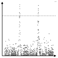
Manhattan plot
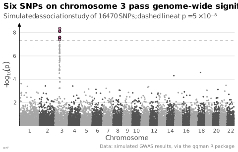
Significance of thousands of tests laid out along a genomic position.
graphique de Manhattan
Significativité de milliers de tests reportée le long d'une position génomique.
L'axe des ordonnées porte le logarithme négatif de la valeur p : les pics sont les signaux.
Classification
- chart
- points and bubbles › scatterplots
- distribution
- the name evokes: building
Channels
 position on common scale; main: −log10 p
 spatial region; main: chromosome
 color hue; main: chromosome (alternating colors)
Attestation
- French term: Common usage, not attested by a source
Scientific literature
OpenAlex: 622 papers since 2010, 54% in the last five years; mostly in Biochemistry, Genetics and Molecular Biology, Medicine, Agricultural and Biological Sciences; Wikidata
R packages
- R
CMplot::CMplot(); GitHub 648 stars; last commit 2026-05; paper (26 citations) - R
qqman::manhattan(); GitHub 175 stars; last commit 2023-08; paper (1 100 citations)
R code of the ggplot2 example
library(ggplot2)
library(dplyr)
library(qqman)
## Simulated association tests along 22 chromosomes, one point per SNP,
## laid end to end; the line marks genome-wide significance (p = 5e-8).
snps <- gwasResults |>
arrange(CHR, BP) |>
mutate(position = row_number(), hit = P < 5e-8,
shade = ifelse(hit, "hit", ifelse(CHR %% 2 == 0, "even", "odd")))
centres <- snps |>
group_by(CHR) |>
summarise(centre = mean(position))
p <- ggplot(snps, aes(x = position, y = -log10(P), colour = shade)) +
geom_hline(yintercept = -log10(5e-8), colour = "#535353", linewidth = 0.3, linetype = "dashed") +
geom_point(data = filter(snps, !hit), size = 0.5) +
## Significant SNPs: black outline, half-transparent fill.
geom_point(data = filter(snps, hit), shape = 21, size = 1.6, colour = "black",
fill = scales::alpha("#9b2367", 0.5), stroke = 0.4) +
scale_colour_manual(values = c(odd = "#a6a6a6", even = "#535353", hit = "#9b2367"), guide = "none") +
scale_x_continuous(breaks = centres$centre[c(1:10, seq(12, 22, 2))],
labels = centres$CHR[c(1:10, seq(12, 22, 2))], expand = expansion(add = 50)) +
scale_y_continuous(expand = expansion(mult = c(0, 0.05))) +
labs(title = "Six SNPs on chromosome 3 pass genome-wide significance",
subtitle = "Simulated association study of 16 470 SNPs; dashed line at p = 5 × 10⁻⁸",
x = "Chromosome", y = expression(-log[10](italic(p))),
caption = "Data: simulated GWAS results, via the qqman R package") +
theme_lex_viz(grid = "y", arrows = "y")Sources (2)
Cite this entry
Stable addresshttps://dataviz.adrientaudiere.com/en/term/manhattan-plot.html
ReferenceTaudière Adrien. 2026. Manhattan plot. In Visualization Vocabulary, version 1.0.0. IdEst. https://dataviz.adrientaudiere.com/en/term/manhattan-plot.html
BibTeX
@incollection{taudiere2026-manhattan-plot,
  author    = {Taudière, Adrien},
  title     = {Manhattan plot},
  booktitle = {Visualization Vocabulary},
  year      = {2026},
  version   = {1.0.0},
  publisher = {IdEst},
  url       = {https://dataviz.adrientaudiere.com/en/term/manhattan-plot.html},
  note      = {CC0 1.0}
}Page created on 2026-10-13. Text last changed on 2026-11-02. Images last changed on 2026-11-12. Numbers computed on 2026-10-22.