
 chart
alluvial plot
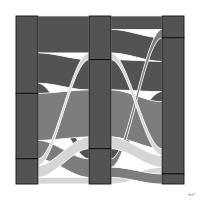
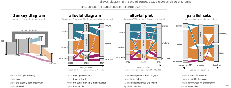
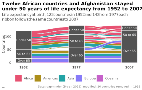
Gapless stacked blocks at each stage of an ordered sequence, crossed by ribbons that each follow the same group of units from the first stage to the last; the height of a column gives the count at that stage.
Classification
- chart
- flows › ribbon flows
- flow, change over time
- the name evokes: nature
Channels
 length; main: count of each group and each path
 area; secondary: count of each group and each path
 spatial region; main: date and group
 color hue; secondary: starting group, kept end to end
Attestation
Seminal references
R packages
R code of the ggplot2 example
library(ggplot2)
library(dplyr)
library(tidyr)
library(ggalluvial)
library(gapminder)
## Countries by life-expectancy band in 1952, 1977 and 2007. As in Brunson
## (2020), each ribbon (geom_alluvium) follows the same countries from one
## date to the next and keeps the color of their continent: one ribbon per
## continent and path.
## Data modified for the example: 20 countries, drawn at random among those
## not named in the title, are removed in 1952 and enter in 1977, so that the
## columns differ in height.
late <- c("Austria", "Chad", "Djibouti", "Equatorial Guinea", "Ethiopia", "Ghana",
"Greece", "Haiti", "Israel", "Myanmar", "Pakistan", "Peru", "Poland",
"Romania", "Sao Tome and Principe", "Sudan", "Sweden", "Switzerland",
"United Kingdom", "Uruguay")
paths <- gapminder |>
filter(year %in% c(1952, 1977, 2007)) |>
mutate(band = cut(lifeExp, c(0, 50, 65, Inf), right = FALSE,
labels = c("Under 50", "50 to 65", "Over 65")),
band = if_else(year == 1952 & country %in% late, NA, band)) |>
select(country, continent, year, band) |>
pivot_wider(names_from = year, values_from = band) |>
count(continent, `1952`, `1977`, `2007`) |>
mutate(path = row_number())
## One row per path and date (lodes form); a path that starts in 1977 has
## no 1952 row, so its ribbon starts there.
lodes <- paths |>
pivot_longer(c(`1952`, `1977`, `2007`), names_to = "year", values_to = "band") |>
filter(!is.na(band))
p <- ggplot(lodes, aes(x = year, stratum = band, alluvium = path, y = n)) +
geom_alluvium(aes(fill = continent), width = 0.3, colour = "white", linewidth = 0.2,
alpha = 0.9) +
geom_stratum(width = 0.3, fill = "#535353", colour = "white", linewidth = 0.3) +
geom_text(stat = "stratum", aes(label = after_stat(stratum)), colour = "white", size = 2.8) +
scale_fill_manual(values = continent_colors) +
scale_x_discrete(expand = expansion(add = 0.2)) +
labs(title = "Twelve African countries and Afghanistan stayed\nunder 50 years of life expectancy from 1952 to 2007",
subtitle = "Life expectancy at birth, 122 countries in 1952 and 142 from 1977;\neach ribbon follows the same countries to 2007",
x = NULL, y = "Countries", fill = NULL,
caption = "Data: gapminder (Bryan 2025), modified: 20 countries removed in 1952") +
theme_lex_viz(grid = "", arrows = "") +
theme(legend.position = "bottom", axis.text.x = element_text(face = "bold"))Sources (1)
Cite this entry
Stable addresshttps://dataviz.adrientaudiere.com/en-only/term/alluvial-plot.html
ReferenceTaudière Adrien. 2026. alluvial plot. In Visualization Vocabulary, version 1.0.0. IdEst. https://dataviz.adrientaudiere.com/en-only/term/alluvial-plot.html
BibTeX
@incollection{taudiere2026-alluvial-plot,
  author    = {Taudière, Adrien},
  title     = {alluvial plot},
  booktitle = {Visualization Vocabulary},
  year      = {2026},
  version   = {1.0.0},
  publisher = {IdEst},
  url       = {https://dataviz.adrientaudiere.com/en-only/term/alluvial-plot.html},
  note      = {CC0 1.0}
}Page created on 2026-11-10. Text last changed on 2026-11-12. Images last changed on 2026-11-11. Numbers computed on 2026-10-22.