
 graphique
 alluvial
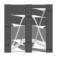
Blocs empilés sans espace à chaque étape d'une suite ordonnée, traversés par des rubans qui suivent chacun le même groupe d'unités de la première étape à la dernière ; la hauteur d'une colonne donne l'effectif de l'étape.
alluvial plot
Gapless stacked blocks at each stage of an ordered sequence, crossed by ribbons that each follow the same group of units from the first stage to the last; the height of a column gives the count at that stage.
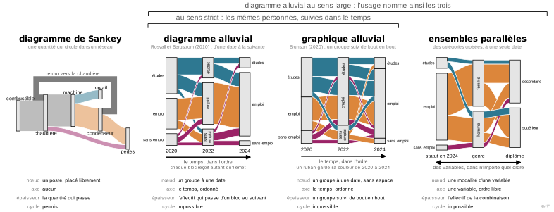
Variante de Brunson (2020), auteur de ggalluvial, qui la range parmi les ensembles parallèles : les modalités gardent le même ordre à chaque étape et s'empilent sans espace, et un ruban (alluvium) garde son identité d'une étape à l'autre, là où le diagramme alluvial de Rosvall et Bergstrom (2010) ne relie que deux étapes voisines. Le nom français est d'usage : guide-R (Larmarange) écrit « graphique alluvial » puis « diagramme alluvial » pour la même figure, sans distinguer les deux noms.
Classification
- graphique
- flux › flux en rubans
- flux, évolution dans le temps
- le nom évoque : nature
Canaux
 longueur; principal : effectif de chaque groupe et de chaque trajectoire
 aire; secondaire : effectif de chaque groupe et de chaque trajectoire
 région de l'espace; principal : date et groupe
 teinte; secondaire : groupe de départ, gardé de bout en bout
Attestation
- terme français : Usage courant, non attesté par une source
- définition anglaise : Brunson, ggalluvial: Layered Grammar for Alluvial Plots, Journal of Open Source Software, 2020↗
Références séminales
Paquets R
Code R de l'exemple ggplot2
library(ggplot2)
library(dplyr)
library(tidyr)
library(ggalluvial)
library(gapminder)
## Countries by life-expectancy band in 1952, 1977 and 2007. As in Brunson
## (2020), each ribbon (geom_alluvium) follows the same countries from one
## date to the next and keeps the color of their continent: one ribbon per
## continent and path.
## Data modified for the example: 20 countries, drawn at random among those
## not named in the title, are removed in 1952 and enter in 1977, so that the
## columns differ in height.
late <- c("Austria", "Chad", "Djibouti", "Equatorial Guinea", "Ethiopia", "Ghana",
"Greece", "Haiti", "Israel", "Myanmar", "Pakistan", "Peru", "Poland",
"Romania", "Sao Tome and Principe", "Sudan", "Sweden", "Switzerland",
"United Kingdom", "Uruguay")
paths <- gapminder |>
filter(year %in% c(1952, 1977, 2007)) |>
mutate(band = cut(lifeExp, c(0, 50, 65, Inf), right = FALSE,
labels = c("Under 50", "50 to 65", "Over 65")),
band = if_else(year == 1952 & country %in% late, NA, band)) |>
select(country, continent, year, band) |>
pivot_wider(names_from = year, values_from = band) |>
count(continent, `1952`, `1977`, `2007`) |>
mutate(path = row_number())
## One row per path and date (lodes form); a path that starts in 1977 has
## no 1952 row, so its ribbon starts there.
lodes <- paths |>
pivot_longer(c(`1952`, `1977`, `2007`), names_to = "year", values_to = "band") |>
filter(!is.na(band))
p <- ggplot(lodes, aes(x = year, stratum = band, alluvium = path, y = n)) +
geom_alluvium(aes(fill = continent), width = 0.3, colour = "white", linewidth = 0.2,
alpha = 0.9) +
geom_stratum(width = 0.3, fill = "#535353", colour = "white", linewidth = 0.3) +
geom_text(stat = "stratum", aes(label = after_stat(stratum)), colour = "white", size = 2.8) +
scale_fill_manual(values = continent_colors) +
scale_x_discrete(expand = expansion(add = 0.2)) +
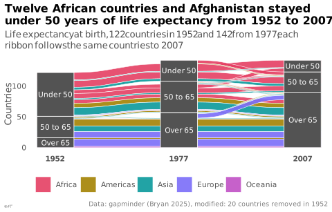
labs(title = "Twelve African countries and Afghanistan stayed\nunder 50 years of life expectancy from 1952 to 2007",
subtitle = "Life expectancy at birth, 122 countries in 1952 and 142 from 1977;\neach ribbon follows the same countries to 2007",
x = NULL, y = "Countries", fill = NULL,
caption = "Data: gapminder (Bryan 2025), modified: 20 countries removed in 1952") +
theme_lex_viz(grid = "", arrows = "") +
theme(legend.position = "bottom", axis.text.x = element_text(face = "bold"))Sources (1)
Citer cette fiche
Adresse stablehttps://dataviz.adrientaudiere.com/terme/alluvial-plot.html
RéférenceTaudière Adrien. 2026. graphique alluvial. Dans Visualization Vocabulary, version 1.0.0. IdEst. https://dataviz.adrientaudiere.com/terme/alluvial-plot.html
BibTeX
@incollection{taudiere2026-alluvial-plot,
  author    = {Taudière, Adrien},
  title     = {graphique alluvial},
  booktitle = {Visualization Vocabulary},
  year      = {2026},
  version   = {1.0.0},
  publisher = {IdEst},
  url       = {https://dataviz.adrientaudiere.com/terme/alluvial-plot.html},
  note      = {CC0 1.0}
}Fiche créée le 10/11/2026. Texte modifié le 12/11/2026. Images modifiées le 11/11/2026. Chiffres calculés le 22/10/2026.