

 chart
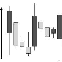
candlestick chart
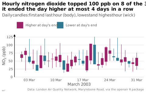
Mark encoding open, close, low and high over a period.
Classification
- chart
- bars › range and target bars
- change over time; Financial Times Visual Vocabulary
- the name evokes: object
Channels
 position on common scale; main: open, close, low, high; time
 length; secondary: range over the period
 color hue; secondary: direction of the variation
Attestation
- English definition: Data Visualisation Guide, data.europa.eu
Scientific literature
OpenAlex: 366 papers since 2000, 49% in the last five years; mostly in Decision Sciences, Economics, Econometrics and Finance, Computer Science; Wikidata
Seminal references
- first known use (1750) Homma, rice trading in Osaka (18th century); Ciuccarelli 2026
- diffusion (1991) Nison (1991). Japanese Candlestick Charting Techniques. New York Institute of Finance; Ciuccarelli 2026
R packages
- R
tidyquant::geom_candlestick(); GitHub 919 stars; last commit 2026-03
R code of the ggplot2 example
library(ggplot2)
library(dplyr)
library(openair)
## One candle per day from the hourly measurements: the first and last hours
## of the day make the body, the lowest and highest hours the wick.
candles <- mydata |>
filter(!is.na(no2), date >= as.POSIXct("2003-03-01", tz = "GMT"),
date < as.POSIXct("2003-04-01", tz = "GMT")) |>
arrange(date) |>
mutate(day = as.Date(date)) |>
group_by(day) |>
summarise(open = first(no2), close = last(no2), low = min(no2), high = max(no2)) |>
mutate(direction = ifelse(close >= open, "Higher at day's end", "Lower at day's end"))
p <- ggplot(candles, aes(x = day)) +
geom_linerange(aes(ymin = low, ymax = high, colour = direction), linewidth = 0.4) +
geom_rect(aes(xmin = day - 0.35, xmax = day + 0.35, ymin = pmin(open, close),
ymax = pmax(open, close), fill = direction)) +
scale_colour_manual(values = unname(lex_colors[c("plum", "blue")]), name = NULL) +
scale_fill_manual(values = unname(lex_colors[c("plum", "blue")]), name = NULL) +
scale_x_date(date_breaks = "1 week", labels = scales::label_date("%d %b", locale = "en")) +
scale_y_continuous(labels = lex_number, limits = c(0, NA), expand = expansion(mult = c(0, 0.05))) +
labs(title = "Hourly nitrogen dioxide topped 100 ppb on 8 of the 31 days;\nit ended the day higher at most 4 days in a row",
subtitle = "Daily candles: first and last hour (body), lowest and highest hour (wick)",
x = "March 2003", y = expression(NO[2]~"(ppb)"),
caption = "Data: London Air Quality Network, Marylebone Road, via the openair R package") +
theme_lex_viz(grid = "y", arrows = "y") +
theme(legend.position = "top")Sources (7)
29 occurrences in the corpus; indexed by 1 book
Cite this entry
Stable addresshttps://dataviz.adrientaudiere.com/en-only/term/candlestick-chart.html
ReferenceTaudière Adrien. 2026. candlestick chart. In Visualization Vocabulary, version 1.0.0. IdEst. https://dataviz.adrientaudiere.com/en-only/term/candlestick-chart.html
BibTeX
@incollection{taudiere2026-candlestick-chart,
  author    = {Taudière, Adrien},
  title     = {candlestick chart},
  booktitle = {Visualization Vocabulary},
  year      = {2026},
  version   = {1.0.0},
  publisher = {IdEst},
  url       = {https://dataviz.adrientaudiere.com/en-only/term/candlestick-chart.html},
  note      = {CC0 1.0}
}Page created on 2026-10-13. Text last changed on 2026-11-10. Images last changed on 2026-11-12. Numbers computed on 2026-10-22.