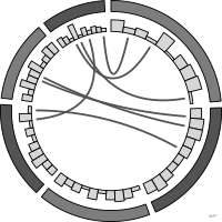
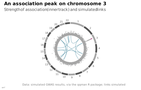
Circos plot

R code of the ggplot2 example

library(ggplot2)
library(dplyr)
library(ggforce)
library(qqman)

## The 22 chromosomes on a circle, each arc as long as its number of SNPs;
## inside, a track of association strength, and links between regions.
## Angles in radians, clockwise from the top (ggforce).
gap <- 0.02
chromosomes <- gwasResults |>
  count(CHR) |>
  mutate(end = cumsum(n * (2 * pi - 22 * gap) / sum(n) + gap) - gap,
         start = end - n * (2 * pi - 22 * gap) / sum(n),
         shade = ifelse(CHR %% 2 == 0, "even", "odd"))
snps <- gwasResults |>
  arrange(CHR, BP) |>
  group_by(CHR) |>
  mutate(rank = row_number()) |>
  ungroup() |>
  left_join(chromosomes, by = "CHR") |>
  mutate(angle = start + (rank - 0.5) / n * (end - start),
         r = 0.55 + 0.4 * -log10(P) / max(-log10(P)),
         hit = P < 5e-8)
## Links between the strongest SNPs of two chromosomes: simulated, for the
## example.
set.seed(4)
top <- slice_min(group_by(snps, CHR), P, n = 1, with_ties = FALSE) |> ungroup()
pairs <- replicate(12, sample(nrow(top), 2))
links <- tibble(from = pairs[1, ], to = pairs[2, ])
link_points <- bind_rows(lapply(seq_len(nrow(links)), function(i) {
  a <- top$angle[links$from[i]]
  b <- top$angle[links$to[i]]
  tibble(id = i, x = c(0.52 * sin(a), 0, 0.52 * sin(b)), y = c(0.52 * cos(a), 0, 0.52 * cos(b)))
}))

p <- ggplot() +
  geom_bezier(data = link_points, aes(x = x, y = y, group = id), colour = "#2e7891",
              alpha = 0.6, linewidth = 0.4) +
  geom_point(data = snps, aes(x = r * sin(angle), y = r * cos(angle), colour = hit), size = 0.15) +
  geom_arc_bar(data = chromosomes, aes(x0 = 0, y0 = 0, r0 = 1, r = 1.07, start = start, end = end,
                                       fill = shade), colour = NA) +
  geom_text(data = chromosomes, aes(x = 1.15 * sin((start + end) / 2), y = 1.15 * cos((start + end) / 2),
                                    label = CHR), size = 2.2, colour = "#535353") +
  scale_fill_manual(values = c(odd = "#a6a6a6", even = "#535353"), guide = "none") +
  scale_colour_manual(values = c(`FALSE` = "#a6a6a6", `TRUE` = "#9b2367"), guide = "none") +
  coord_equal(xlim = c(-2, 2), ylim = c(-1.2, 1.2), clip = "off") +
  labs(title = "An association peak on chromosome 3",
       subtitle = "Strength of association (inner track) and simulated links",
       x = NULL, y = NULL,
       caption = "Data: simulated GWAS results, via the qqman R package; links simulated") +
  theme_lex_viz(grid = "", arrows = "") +
  theme(axis.text = element_blank())