
 map
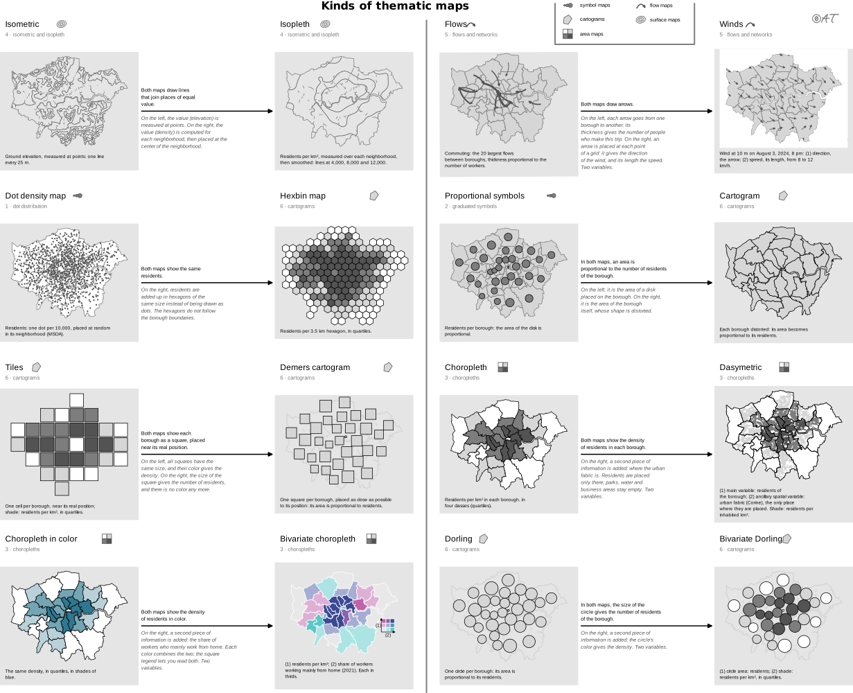
dasymetric map
also: dasymetric mapping“A technique in which attribute data that is organized by a large or arbitrary area unit is more accurately distributed within that unit by the overlay of geographic boundaries that exclude, restrict, or confine the attribute in question.”
Classification
- map
- maps › area maps
- spatial
Attestation
- English definition: Esri, GIS Dictionary↗
Scientific literature
OpenAlex: 56 papers since 2005, 21% in the last five years; mostly in Social Sciences, Environmental Science, Computer Science; Wikidata
Seminal references
- first known use (1833) Scrope (1833). Principles of Political Economy, deduced from the natural laws of social welfare, and applied to the present state of Britain (population density map); Friendly & Denis 2001
- formalization (1936) Wright (1936). A Method of Mapping Densities of Population: With Cape Cod as an Example. Geographical Review, 26(1), 103 (276 citations)
R code of the ggplot2 example
library(ggplot2)
library(dplyr)
library(sf)
library(patchwork)
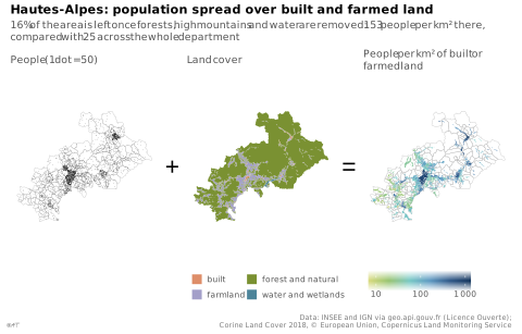
## Communes of the Hautes-Alpes, their land cover (Corine Land Cover 2018) and
## their built or farmed land, prepared by tools/donnees_dasymetrique.R.
gpkg <- "illustrations/ggplot/data/dasymetric-map.gpkg"
communes <- st_read(gpkg, "communes", quiet = TRUE)
land <- st_read(gpkg, "occupation", quiet = TRUE)
habitable <- st_read(gpkg, "habitable", quiet = TRUE) |>
left_join(st_drop_geometry(communes), by = "code") |>
mutate(density = population / (as.numeric(st_area(geom)) / 1e6))
## One dot for 50 people, drawn anywhere in its commune: all that is known
## before the land cover is brought in.
set.seed(1)
dots <- st_sample(communes, size = round(communes$population / 50))
borders <- geom_sf(data = communes, fill = NA, colour = "grey70", linewidth = 0.1)
## The theme goes to each map, not to the whole: the "+" and "=" stay bare.
map <- function(p, legend = "none") {
p + coord_sf(datum = NA) +
theme_lex_viz(base_size = 7, grid = "", arrows = "") +
theme(legend.position = legend, legend.key.size = unit(2.5, "mm"))
}
p1 <- map(ggplot() + borders + geom_sf(data = dots, size = 0.15, shape = 16, stroke = 0) +
labs(subtitle = "People (1 dot = 50)"))
## Four of the Rattner colors, each given to the land cover it evokes.
p2 <- map(ggplot() +
geom_sf(data = land, aes(fill = groupe), colour = NA) +
scale_fill_manual(values = c(built = "#de8e69", farmland = "#a39fc9",
`forest and natural` = "#7a9132",
`water and wetlands` = "#4c849a")) +
guides(fill = guide_legend(ncol = 2)) +
labs(subtitle = "Land cover", fill = NULL), "bottom")
p3 <- map(ggplot() + borders +
geom_sf(data = habitable, aes(fill = density), colour = NA) +
scale_fill_continuous(transform = "log10", breaks = c(10, 100, 1000),
labels = lex_number) +
guides(fill = guide_colourbar(barwidth = unit(25, "mm"))) +
labs(subtitle = "People per km² of built or farmed land", fill = NULL), "bottom")
sign <- function(s) {
ggplot() + annotate("text", x = 0, y = 0, label = s, size = 6) + theme_void()
}
p <- p1 + sign("+") + p2 + sign("=") + p3 +
plot_layout(nrow = 1, widths = c(1, 0.12, 1, 0.12, 1)) +
plot_annotation(
title = "Hautes-Alpes: population spread over built and farmed land",
subtitle = "16% of the area is left once forests, high mountains and water are removed: 153 people per km² there, compared with 25 across the whole department",
caption = "Data: INSEE and IGN via geo.api.gouv.fr (Licence Ouverte);\nCorine Land Cover 2018, © European Union, Copernicus Land Monitoring Service",
theme = theme_lex_viz(base_size = 7, grid = "", arrows = "")
)Sources (9)
130 occurrences in the corpus; indexed by 3 books
- Atlas of knowledge: anyone can map
- Cartography: thematic map design
- Data visualisation: a handbook for data driven design
- Data visualization handbook
- Esri, GIS Dictionary↗
- Interactive data visualization: foundations, techniques, and applications
- Milestones in the history of thematic cartography, statistical graphics, and data visua...
- Thematic Cartography and Geovisualization
- Wikipedia in English↗
Cite this entry
Stable addresshttps://dataviz.adrientaudiere.com/en-only/term/dasymetric-map.html
ReferenceTaudière Adrien. 2026. dasymetric map. In Visualization Vocabulary, version 1.0.0. IdEst. https://dataviz.adrientaudiere.com/en-only/term/dasymetric-map.html
BibTeX
@incollection{taudiere2026-dasymetric-map,
  author    = {Taudière, Adrien},
  title     = {dasymetric map},
  booktitle = {Visualization Vocabulary},
  year      = {2026},
  version   = {1.0.0},
  publisher = {IdEst},
  url       = {https://dataviz.adrientaudiere.com/en-only/term/dasymetric-map.html},
  note      = {CC0 1.0}
}Page created on 2026-11-03. Text last changed on 2026-11-10. Images last changed on 2026-11-12. Numbers computed on 2026-10-22.