
 map
dasymetric map
also: dasymetric mapping“A technique in which attribute data that is organized by a large or arbitrary area unit is more accurately distributed within that unit by the overlay of geographic boundaries that exclude, restrict, or confine the attribute in question.”
dasymetric map
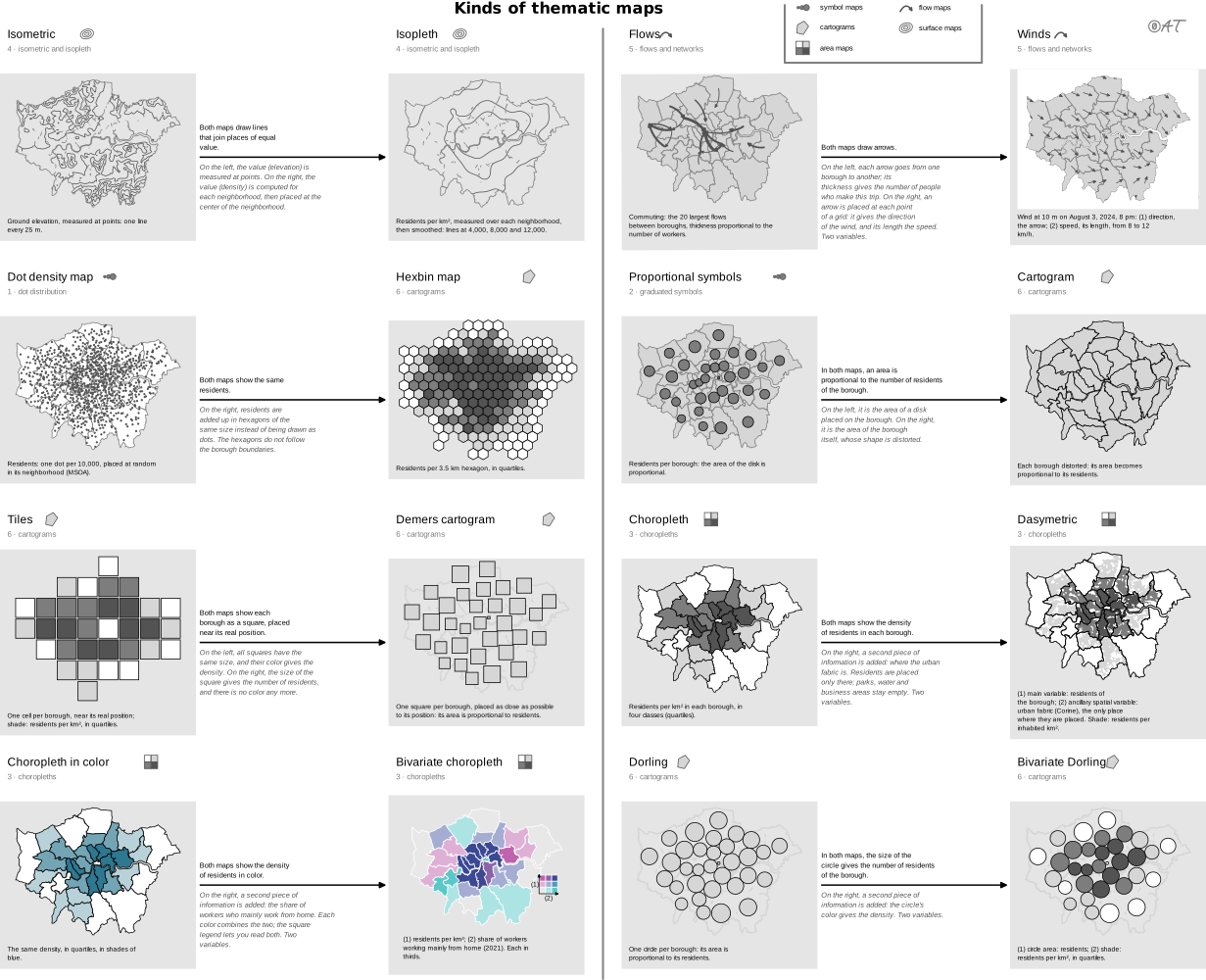
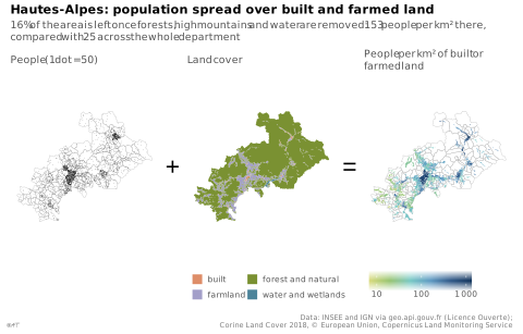
Carte qui répartit plus finement une première variable grâce à une autre variable spatiale qui a un lien logique, parfois en retirant les zones où cette première variable ne peut pas se trouver.
Sert presque toujours à la densité de population : on retire des unités l'eau, les forêts et les terres agricoles. Börner la décrit comme un hybride de la choroplèthe et de la carte isarithmique. Nom anglais gardé en français (choix du développeur). Définition anglaise : version du GIS Dictionary d’Esri archivée en 2015 (la page actuelle la reformule).
Classification
- map
- maps › area maps
- spatial
Attestation
- French term: Common usage, not attested by a source
- English definition: Esri, GIS Dictionary↗
Scientific literature
OpenAlex: 56 papers since 2005, 21% in the last five years; mostly in Social Sciences, Environmental Science, Computer Science; Wikidata
Seminal references
- first known use (1833) Scrope (1833). Principles of Political Economy, deduced from the natural laws of social welfare, and applied to the present state of Britain (population density map); Friendly & Denis 2001
- formalization (1936) Wright (1936). A Method of Mapping Densities of Population: With Cape Cod as an Example. Geographical Review, 26(1), 103 (276 citations)
R code of the ggplot2 example
library(ggplot2)
library(dplyr)
library(sf)
library(patchwork)
## Communes of the Hautes-Alpes, their land cover (Corine Land Cover 2018) and
## their built or farmed land, prepared by tools/donnees_dasymetrique.R.
gpkg <- "illustrations/ggplot/data/dasymetric-map.gpkg"
communes <- st_read(gpkg, "communes", quiet = TRUE)
land <- st_read(gpkg, "occupation", quiet = TRUE)
habitable <- st_read(gpkg, "habitable", quiet = TRUE) |>
left_join(st_drop_geometry(communes), by = "code") |>
mutate(density = population / (as.numeric(st_area(geom)) / 1e6))
## One dot for 50 people, drawn anywhere in its commune: all that is known
## before the land cover is brought in.
set.seed(1)
dots <- st_sample(communes, size = round(communes$population / 50))
borders <- geom_sf(data = communes, fill = NA, colour = "grey70", linewidth = 0.1)
## The theme goes to each map, not to the whole: the "+" and "=" stay bare.
map <- function(p, legend = "none") {
p + coord_sf(datum = NA) +
theme_lex_viz(base_size = 7, grid = "", arrows = "") +
theme(legend.position = legend, legend.key.size = unit(2.5, "mm"))
}
p1 <- map(ggplot() + borders + geom_sf(data = dots, size = 0.15, shape = 16, stroke = 0) +
labs(subtitle = "People (1 dot = 50)"))
## Four of the Rattner colors, each given to the land cover it evokes.
p2 <- map(ggplot() +
geom_sf(data = land, aes(fill = groupe), colour = NA) +
scale_fill_manual(values = c(built = "#de8e69", farmland = "#a39fc9",
`forest and natural` = "#7a9132",
`water and wetlands` = "#4c849a")) +
guides(fill = guide_legend(ncol = 2)) +
labs(subtitle = "Land cover", fill = NULL), "bottom")
p3 <- map(ggplot() + borders +
geom_sf(data = habitable, aes(fill = density), colour = NA) +
scale_fill_continuous(transform = "log10", breaks = c(10, 100, 1000),
labels = lex_number) +
guides(fill = guide_colourbar(barwidth = unit(25, "mm"))) +
labs(subtitle = "People per km² of built or farmed land", fill = NULL), "bottom")
sign <- function(s) {
ggplot() + annotate("text", x = 0, y = 0, label = s, size = 6) + theme_void()
}
p <- p1 + sign("+") + p2 + sign("=") + p3 +
plot_layout(nrow = 1, widths = c(1, 0.12, 1, 0.12, 1)) +
plot_annotation(
title = "Hautes-Alpes: population spread over built and farmed land",
subtitle = "16% of the area is left once forests, high mountains and water are removed: 153 people per km² there, compared with 25 across the whole department",
caption = "Data: INSEE and IGN via geo.api.gouv.fr (Licence Ouverte);\nCorine Land Cover 2018, © European Union, Copernicus Land Monitoring Service",
theme = theme_lex_viz(base_size = 7, grid = "", arrows = "")
)Sources (9)
130 occurrences in the corpus; indexed by 3 books
- Atlas of knowledge: anyone can map
- Cartography: thematic map design
- Data visualisation: a handbook for data driven design
- Data visualization handbook
- Esri, GIS Dictionary↗
- Interactive data visualization: foundations, techniques, and applications
- Milestones in the history of thematic cartography, statistical graphics, and data visua...
- Thematic Cartography and Geovisualization
- Wikipedia in English↗
Cite this entry
Stable addresshttps://dataviz.adrientaudiere.com/en/term/dasymetric-map.html
ReferenceTaudière Adrien. 2026. dasymetric map. In Visualization Vocabulary, version 1.0.0. IdEst. https://dataviz.adrientaudiere.com/en/term/dasymetric-map.html
BibTeX
@incollection{taudiere2026-dasymetric-map,
  author    = {Taudière, Adrien},
  title     = {dasymetric map},
  booktitle = {Visualization Vocabulary},
  year      = {2026},
  version   = {1.0.0},
  publisher = {IdEst},
  url       = {https://dataviz.adrientaudiere.com/en/term/dasymetric-map.html},
  note      = {CC0 1.0}
}Page created on 2026-11-03. Text last changed on 2026-11-10. Images last changed on 2026-11-12. Numbers computed on 2026-10-22.