
 chart
ternary plot
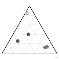
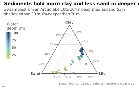
Scatterplot drawn in a triangle, where each point's position gives the shares of three components of a single whole.
diagramme ternaire
Nuage de points tracé dans un triangle, où la position de chaque point donne les parts de trois composantes d'un même tout.
Kirk 2019 et Koponen 2019 en font une variante du nuage de points. Courant en géologie (triangle des textures des sols) et en métallurgie ; en génétique des populations, c'est le diagramme de De Finetti.
Classification
- chart
- points and bubbles › scatterplots
- part-to-whole
Channels
 position on common scale; main: three parts of a whole
 color hue; secondary: group
Attestation and synonyms
- French term: French Wikipedia↗
- English definition: Koponen & Hildén, Data Visualization Handbook, Aalto, 2019
- graphique triangulaire; Bertin, Sémiologie graphique, 1967
- diagramme triangulaire; Bertin, Sémiologie graphique, 1967
- représentation triangulaire; PBIL biostatistics notes (Chessel, Dufour, Thioulouse et al., Lyon 1)
- trilinear chart; Brinton, Graphic Presentation, 1939↗
- trilinear graph; Information Graphics: A Comprehensive Illustrated Reference
- triangular coordinates plot; Wilkinson, The Grammar of Graphics, 2nd ed., 2005
- ternary chart; Questions in Dataviz: A Design-Driven Process for Data Visualisation
- ternary diagram; Cook & Laa, Interactively Exploring High-Dimensional Data and Models in R, Chapman & Hall/CRC, 2026
- ternary graph; Wikipedia in English↗
- simplex plot; Wikipedia in English↗
Scientific literature
OpenAlex: 760 papers since 1968, 36% in the last five years; mostly in Earth and Planetary Sciences, Environmental Science, Agricultural and Biological Sciences; Wikidata
Seminal references
R packages
- R
Ternary::TernaryPlot(); GitHub; paper Graphisme de base R ; trace aussi les diagrammes de Holdridge. - R
ade4::triangle.plot(); GitHub; paper La « représentation triangulaire » des fiches du PBIL. - R
ggtern::ggtern(); paper Extension de ggplot2 (coord_tern). DOI de l'article de Hamilton & Ferry 2018 (JSS) ; celui du paquet est 10.32614/CRAN.package.ggtern.
R code of the ggplot2 example
library(ggplot2)
## Sand, silt and clay of 39 sediment samples taken at different water depths
## in an Arctic lake (Aitchison 1986). Plain ggplot2: each composition is
## projected into an equilateral triangle, sand bottom left, silt bottom
## right, clay on top.
data(ArcticLake, package = "compositions")
lake <- as.data.frame(ArcticLake)
lake[c("sand", "silt", "clay")] <- lake[c("sand", "silt", "clay")] / rowSums(lake[c("sand", "silt", "clay")])
to_xy <- function(sand, silt, clay) {
data.frame(x = silt + clay / 2, y = clay * sqrt(3) / 2)
}
lake <- cbind(lake, to_xy(lake$sand, lake$silt, lake$clay))
## Grid lines every 20%, one family per component. Each line ends on the
## side where it is read, and a short tick prolongs it outside the triangle:
## clay on the left side, sand at the bottom, silt on the right side.
s <- seq(0.2, 0.8, by = 0.2)
ends <- function(read_at, other_end) {
setNames(cbind(read_at, other_end), c("x", "y", "xend", "yend"))
}
grid_lines <- rbind(
ends(to_xy(1 - s, 0, s), to_xy(0, 1 - s, s)), # clay
ends(to_xy(s, 1 - s, 0), to_xy(s, 0, 1 - s)), # sand
ends(to_xy(0, s, 1 - s), to_xy(1 - s, s, 0)) # silt
)
grid_lines$hj <- rep(c(1, 0, 0), each = length(s))
grid_lines$vj <- rep(c(0.5, 1, 0), each = length(s))
grid_lines$label <- paste0(s * 100, "%")
## Outward direction of each line at the end where it is read.
len <- with(grid_lines, sqrt((x - xend)^2 + (y - yend)^2))
grid_lines$dx <- with(grid_lines, (x - xend) / len)
grid_lines$dy <- with(grid_lines, (y - yend) / len)
tick <- 0.035
frame <- to_xy(c(1, 0, 0, 1), c(0, 1, 0, 0), c(0, 0, 1, 0))
vertices <- cbind(to_xy(c(1, 0, 0), c(0, 1, 0), c(0, 0, 1)),
label = c("Sand", "Silt", "Clay"),
hj = c(1.15, -0.15, 0.5), vj = c(0.5, 0.5, -0.6))
p <- ggplot(lake, aes(x, y)) +
geom_segment(data = grid_lines, aes(xend = xend, yend = yend),
colour = "#d6d6d6", linewidth = 0.25) +
geom_segment(data = grid_lines, aes(xend = x + tick * dx, yend = y + tick * dy),
colour = "#535353", linewidth = 0.3) +
geom_text(data = grid_lines, aes(x + 1.3 * tick * dx, y + 1.3 * tick * dy,
label = label, hjust = hj, vjust = vj),
colour = "#7d7d7d", size = 2.3) +
geom_path(data = frame, colour = "#535353", linewidth = 0.5) +
geom_point(aes(fill = depth), shape = 21, size = 2, colour = "#535353", stroke = 0.25) +
geom_text(data = vertices, aes(label = label, hjust = hj, vjust = vj),
colour = "#535353", size = 3.2, fontface = "bold") +
scale_fill_gradientn(colours = idest_seq, labels = lex_number) +
coord_equal(xlim = c(-0.55, 1.55), ylim = c(-0.08, 0.9), clip = "off") +
labs(title = "Sediments hold more clay and less sand in deeper water",
subtitle = "39 samples from an Arctic lake, 10 to 104 m deep; median sand: 53% shallower than 30 m, 6% deeper than 70 m",
fill = "Water\ndepth (m)",
caption = "Data: Aitchison 1986, via the compositions R package") +
theme_lex_viz(grid = "", arrows = "") +
theme(axis.text = element_blank(), axis.title = element_blank(),
legend.position = "inside", legend.position.inside = c(0, 1),
legend.justification.inside = c(0, 1), legend.key.height = unit(5, "mm"),
legend.key.width = unit(3, "mm"))Sources (13)
10 occurrences in the corpus; indexed by 2 books
Show the 13 sources
- Cook & Laa, Interactively Exploring High-Dimensional Data and Models in R, Chapman & Hall/CRC, 2026
- Data Visualisation Guide, data.europa.eu
- Data visualisation: a handbook for data driven design
- Data visualization handbook
- Data Viz Project
- dataphys.org
- datavizproject.com
- French Wikipedia↗
- Koponen & Hildén, Data Visualization Handbook, Aalto, 2019
- LibreTexts Statistics, textbook chapters on charts
- Magrit user manual, French version (UAR RIATE, CNRS)
- Visualizing with text
- Wikipedia in English↗
Cite this entry
Stable addresshttps://dataviz.adrientaudiere.com/en/term/ternary-plot.html
ReferenceTaudière Adrien. 2026. ternary plot. In Visualization Vocabulary, version 1.0.0. IdEst. https://dataviz.adrientaudiere.com/en/term/ternary-plot.html
BibTeX
@incollection{taudiere2026-ternary-plot,
  author    = {Taudière, Adrien},
  title     = {ternary plot},
  booktitle = {Visualization Vocabulary},
  year      = {2026},
  version   = {1.0.0},
  publisher = {IdEst},
  url       = {https://dataviz.adrientaudiere.com/en/term/ternary-plot.html},
  note      = {CC0 1.0}
}Page created on 2026-11-09. Text last changed on 2026-11-10. Images last changed on 2026-11-11. Numbers computed on 2026-10-22.