
 graphique
diagramme ternaire
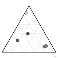
Nuage de points tracé dans un triangle, où la position de chaque point donne les parts de trois composantes d'un même tout.
ternary plot
Scatterplot drawn in a triangle, where each point's position gives the shares of three components of a single whole.
Kirk 2019 et Koponen 2019 en font une variante du nuage de points. Courant en géologie (triangle des textures des sols) et en métallurgie ; en génétique des populations, c'est le diagramme de De Finetti.
Classification
- graphique
- points et bulles › nuages de points
- partie d'un tout
Canaux
 position sur une échelle commune; principal : trois parts d'un tout
 teinte; secondaire : groupe
Attestation et synonymies
- terme français : Wikipédia en français↗
- définition anglaise : Koponen & Hildén, Data Visualization Handbook, Aalto, 2019
- graphique triangulaire; Bertin, Sémiologie graphique, 1967
- diagramme triangulaire; Bertin, Sémiologie graphique, 1967
- représentation triangulaire; Fiches de biostatistique du PBIL (Chessel, Dufour, Thioulouse et al., Lyon 1)
- trilinear chart; Brinton, Graphic Presentation, 1939↗
- trilinear graph; Information Graphics: A Comprehensive Illustrated Reference
- triangular coordinates plot; Wilkinson, The Grammar of Graphics, 2e éd., 2005
- ternary chart; Questions in Dataviz: A Design-Driven Process for Data Visualisation
- ternary diagram; Cook & Laa, Interactively Exploring High-Dimensional Data and Models in R, Chapman & Hall/CRC, 2026
- ternary graph; Wikipedia in English↗
- simplex plot; Wikipedia in English↗
Littérature scientifique
OpenAlex : 760 articles depuis 1968, dont 36 % ces cinq dernières années; surtout en Earth and Planetary Sciences, Environmental Science, Agricultural and Biological Sciences; Wikidata
Références séminales
Paquets R
- R
Ternary::TernaryPlot(); GitHub; article Graphisme de base R ; trace aussi les diagrammes de Holdridge. - R
ade4::triangle.plot(); GitHub; article La « représentation triangulaire » des fiches du PBIL. - R
ggtern::ggtern(); article Extension de ggplot2 (coord_tern). DOI de l'article de Hamilton & Ferry 2018 (JSS) ; celui du paquet est 10.32614/CRAN.package.ggtern.
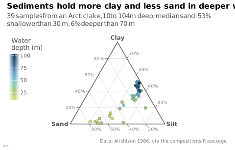
Code R de l'exemple ggplot2
library(ggplot2)
## Sand, silt and clay of 39 sediment samples taken at different water depths
## in an Arctic lake (Aitchison 1986). Plain ggplot2: each composition is
## projected into an equilateral triangle, sand bottom left, silt bottom
## right, clay on top.
data(ArcticLake, package = "compositions")
lake <- as.data.frame(ArcticLake)
lake[c("sand", "silt", "clay")] <- lake[c("sand", "silt", "clay")] / rowSums(lake[c("sand", "silt", "clay")])
to_xy <- function(sand, silt, clay) {
data.frame(x = silt + clay / 2, y = clay * sqrt(3) / 2)
}
lake <- cbind(lake, to_xy(lake$sand, lake$silt, lake$clay))
## Grid lines every 20%, one family per component. Each line ends on the
## side where it is read, and a short tick prolongs it outside the triangle:
## clay on the left side, sand at the bottom, silt on the right side.
s <- seq(0.2, 0.8, by = 0.2)
ends <- function(read_at, other_end) {
setNames(cbind(read_at, other_end), c("x", "y", "xend", "yend"))
}
grid_lines <- rbind(
ends(to_xy(1 - s, 0, s), to_xy(0, 1 - s, s)), # clay
ends(to_xy(s, 1 - s, 0), to_xy(s, 0, 1 - s)), # sand
ends(to_xy(0, s, 1 - s), to_xy(1 - s, s, 0)) # silt
)
grid_lines$hj <- rep(c(1, 0, 0), each = length(s))
grid_lines$vj <- rep(c(0.5, 1, 0), each = length(s))
grid_lines$label <- paste0(s * 100, "%")
## Outward direction of each line at the end where it is read.
len <- with(grid_lines, sqrt((x - xend)^2 + (y - yend)^2))
grid_lines$dx <- with(grid_lines, (x - xend) / len)
grid_lines$dy <- with(grid_lines, (y - yend) / len)
tick <- 0.035
frame <- to_xy(c(1, 0, 0, 1), c(0, 1, 0, 0), c(0, 0, 1, 0))
vertices <- cbind(to_xy(c(1, 0, 0), c(0, 1, 0), c(0, 0, 1)),
label = c("Sand", "Silt", "Clay"),
hj = c(1.15, -0.15, 0.5), vj = c(0.5, 0.5, -0.6))
p <- ggplot(lake, aes(x, y)) +
geom_segment(data = grid_lines, aes(xend = xend, yend = yend),
colour = "#d6d6d6", linewidth = 0.25) +
geom_segment(data = grid_lines, aes(xend = x + tick * dx, yend = y + tick * dy),
colour = "#535353", linewidth = 0.3) +
geom_text(data = grid_lines, aes(x + 1.3 * tick * dx, y + 1.3 * tick * dy,
label = label, hjust = hj, vjust = vj),
colour = "#7d7d7d", size = 2.3) +
geom_path(data = frame, colour = "#535353", linewidth = 0.5) +
geom_point(aes(fill = depth), shape = 21, size = 2, colour = "#535353", stroke = 0.25) +
geom_text(data = vertices, aes(label = label, hjust = hj, vjust = vj),
colour = "#535353", size = 3.2, fontface = "bold") +
scale_fill_gradientn(colours = idest_seq, labels = lex_number) +
coord_equal(xlim = c(-0.55, 1.55), ylim = c(-0.08, 0.9), clip = "off") +
labs(title = "Sediments hold more clay and less sand in deeper water",
subtitle = "39 samples from an Arctic lake, 10 to 104 m deep; median sand: 53% shallower than 30 m, 6% deeper than 70 m",
fill = "Water\ndepth (m)",
caption = "Data: Aitchison 1986, via the compositions R package") +
theme_lex_viz(grid = "", arrows = "") +
theme(axis.text = element_blank(), axis.title = element_blank(),
legend.position = "inside", legend.position.inside = c(0, 1),
legend.justification.inside = c(0, 1), legend.key.height = unit(5, "mm"),
legend.key.width = unit(3, "mm"))Sources (13)
10 occurrences dans le corpus; indexé par 2 ouvrages
Afficher les 13 sources
- Cook & Laa, Interactively Exploring High-Dimensional Data and Models in R, Chapman & Hall/CRC, 2026
- Data Visualisation Guide, data.europa.eu
- Data visualisation: a handbook for data driven design
- Data visualization handbook
- Data Viz Project
- dataphys.org
- datavizproject.com
- Koponen & Hildén, Data Visualization Handbook, Aalto, 2019
- LibreTexts Statistics, chapitres de manuels sur les figures
- Magrit, manuel d'utilisation (UAR RIATE, CNRS)
- Visualizing with text
- Wikipédia en français↗
- Wikipedia in English↗
Citer cette fiche
Adresse stablehttps://dataviz.adrientaudiere.com/terme/ternary-plot.html
RéférenceTaudière Adrien. 2026. diagramme ternaire. Dans Visualization Vocabulary, version 1.0.0. IdEst. https://dataviz.adrientaudiere.com/terme/ternary-plot.html
BibTeX
@incollection{taudiere2026-ternary-plot,
  author    = {Taudière, Adrien},
  title     = {diagramme ternaire},
  booktitle = {Visualization Vocabulary},
  year      = {2026},
  version   = {1.0.0},
  publisher = {IdEst},
  url       = {https://dataviz.adrientaudiere.com/terme/ternary-plot.html},
  note      = {CC0 1.0}
}Fiche créée le 09/11/2026. Texte modifié le 10/11/2026. Images modifiées le 11/11/2026. Chiffres calculés le 22/10/2026.