
 graphique
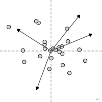
biplot
aussi : double projectionProjection simultanée des individus et des variables d'une ordination.
biplot
Simultaneous projection of individuals and variables of an ordination.
Classification
- graphique
- points et bulles › nuages de points
- corrélation
Canaux
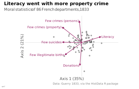
 position sur une échelle commune; principal : coordonnées des individus
 longueur; principal : contribution de la variable (longueur des flèches)
 inclinaison ou angle; principal : direction de la variable (flèches)
 teinte; secondaire : groupe
Attestation
- terme français : Rakotomalala, fascicules de cours de statistique (Université Lyon 2)
Littérature scientifique
OpenAlex : 8 880 articles depuis 1970, dont 41 % ces cinq dernières années; surtout en Agricultural and Biological Sciences, Mathematics, Environmental Science; Wikidata
Références séminales
- invention (1971) GABRIEL (1971). The biplot graphic display of matrices with application to principal component analysis. Biometrika (3 088 citations); Friendly & Denis 2001
Paquets R
- R
factoextra::fviz_pca_biplot(); GitHub 389 étoiles; dernier commit 2026-07 - R
FactoMineR::plot.PCA(); GitHub 59 étoiles; dernier commit 2026-09; article (11 669 citations) Cartes des individus et des variables après PCA(). - R
ade4::scatter(); GitHub 46 étoiles; dernier commit 2026-01; article (6 235 citations) Biplot d'une analyse factorielle (objet dudi) : individus et variables.
Code R de l'exemple ggplot2
library(ggplot2)
library(HistData)
## Guerry's moral statistics are scaled so that more is better: crimes,
## illegitimate births and suicides are counted as population per event.
## The arrow names say so.
moral <- c(Crime_pers = "Few crimes (persons)", Crime_prop = "Few crimes (property)",
Literacy = "Literacy", Donations = "Donations",
Infants = "Few illegitimate births", Suicides = "Few suicides")
pca <- prcomp(Guerry[, names(moral)], scale. = TRUE)
share <- scales::percent(pca$sdev^2 / sum(pca$sdev^2), accuracy = 1)
departments <- as.data.frame(pca$x[, 1:2])
## Arrows stretched to the spread of the departments, so both read on one plot.
stretch <- max(abs(pca$x[, 1:2])) / max(abs(pca$rotation[, 1:2])) * 0.8
variables <- data.frame(pca$rotation[, 1:2] * stretch, name = moral[rownames(pca$rotation)])
p <- ggplot(departments, aes(x = PC1, y = PC2)) +
geom_hline(yintercept = 0, colour = "#d6d6d6", linewidth = 0.3) +
geom_vline(xintercept = 0, colour = "#d6d6d6", linewidth = 0.3) +
geom_point(size = 1.2, alpha = 0.5, colour = "#535353") +
geom_segment(data = variables, aes(x = 0, y = 0, xend = PC1, yend = PC2),
colour = "#9b2367", linewidth = 0.5,
arrow = grid::arrow(length = unit(1.6, "mm"), angle = 25, type = "closed")) +
geom_text(data = variables, aes(label = name), colour = "#9b2367", size = 2.8,
hjust = ifelse(variables$PC1 > 0, 0, 1), nudge_x = ifelse(variables$PC1 > 0, 0.1, -0.1)) +
scale_x_continuous(labels = lex_number, expand = expansion(mult = c(0.6, 0.35))) +
scale_y_continuous(labels = lex_number, expand = expansion(mult = 0.1)) +
coord_fixed(clip = "off") +
labs(title = "Literacy went with more property crime",
subtitle = "Moral statistics of 86 French departments, 1833",
x = paste0("Axis 1 (", share[1], ")"), y = paste0("Axis 2 (", share[2], ")"),
caption = "Data: Guerry 1833, via the HistData R package") +
theme_lex_viz(grid = "", arrows = "") +
theme(axis.text = element_blank())Sources (11)
55 occurrences dans le corpus; indexé par 4 ouvrages
Afficher les 11 sources
- Applied Multivariate Statistics in R
- Cook & Laa, Interactively Exploring High-Dimensional Data and Models in R, Chapman & Hall/CRC, 2026
- Fiches de biostatistique du PBIL (Chessel, Dufour, Thioulouse et al., Lyon 1)
- Grosjean & Engels, Science des données biologiques I-III (Université de Mons)
- How maps work: representation, visualization, and design
- Milestones in the history of thematic cartography, statistical graphics, and data visua...
- Rakotomalala, fascicules de cours de statistique (Université Lyon 2)
- Série d'ateliers R du CSBQ, version française (Centre de la science de la biodiversité du Québec)
- The grammar of graphics
- utilitR, documentation collaborative sur R (Insee)
- Wikipedia in English↗
Citer cette fiche
Adresse stablehttps://dataviz.adrientaudiere.com/terme/biplot.html
RéférenceTaudière Adrien. 2026. biplot. Dans Visualization Vocabulary, version 1.0.0. IdEst. https://dataviz.adrientaudiere.com/terme/biplot.html
BibTeX
@incollection{taudiere2026-biplot,
  author    = {Taudière, Adrien},
  title     = {biplot},
  booktitle = {Visualization Vocabulary},
  year      = {2026},
  version   = {1.0.0},
  publisher = {IdEst},
  url       = {https://dataviz.adrientaudiere.com/terme/biplot.html},
  note      = {CC0 1.0}
}Fiche créée le 13/10/2026. Texte modifié le 22/10/2026. Images modifiées le 12/11/2026. Chiffres calculés le 22/10/2026.