

 encodage
coordonnées polaires
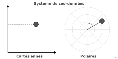
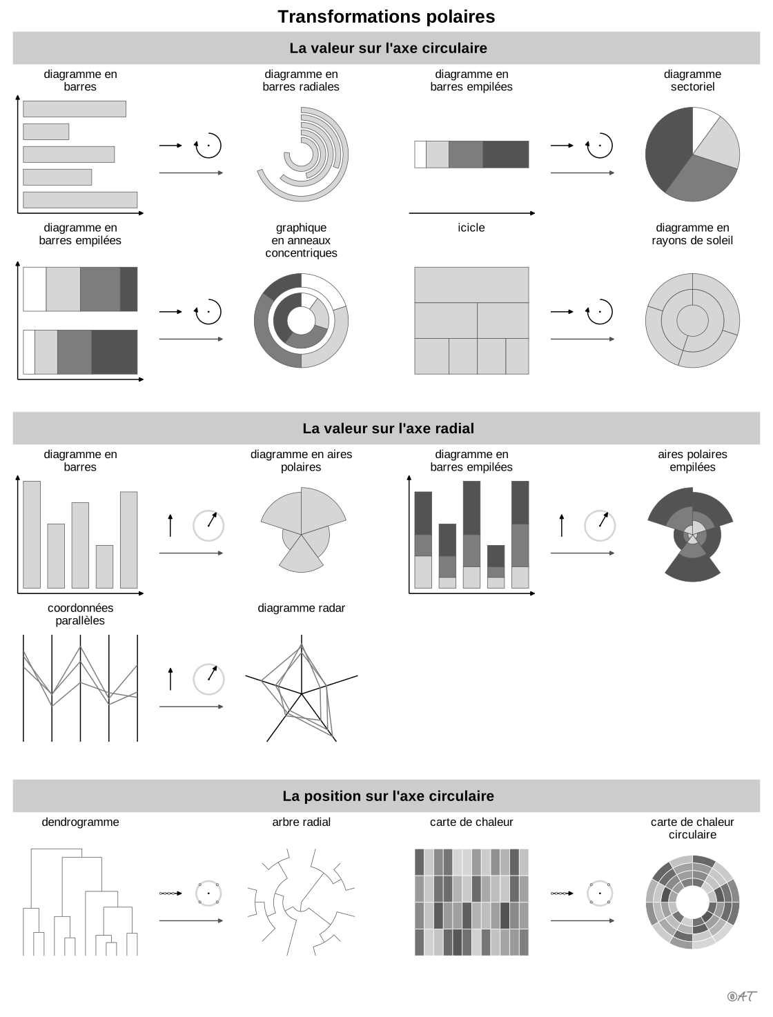
aussi : repère polaireRepère où la position est donnée par un angle et un rayon.
polar coordinates
Frame where position is given by an angle and a radius.
Classification
- encodage
Attestation
- terme français : Lagnel, Manuel de datavisualisation, Dunod, 2021
- définition anglaise : Référence de ggplot2
Code R de l'exemple ggplot2
library(ggplot2)
library(patchwork)
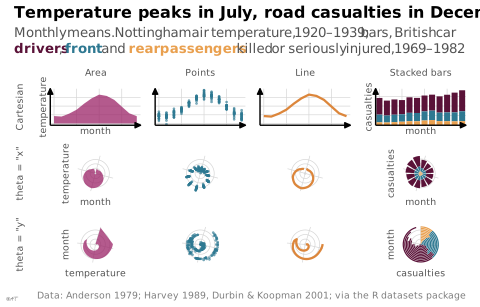
## A monthly cycle drawn as an area, as points, as a line and as stacked
## bars, in Cartesian coordinates, then through coord_radial() with either
## axis as the angle. Area, points and line: air temperature at Nottingham,
## 1920-1939, converted from Fahrenheit. Stacked bars: car occupants killed
## or seriously injured in Great Britain, before the seat-belt law of 1983;
## counts add up, which temperatures do not.
monthly <- data.frame(month = as.numeric(cycle(nottem)),
temp = (as.numeric(nottem) - 32) * 5 / 9)
mean_temp <- aggregate(temp ~ month, monthly, mean)
seats <- data.frame(month = as.numeric(cycle(Seatbelts)),
year = floor(as.numeric(time(Seatbelts))),
Seatbelts[, c("drivers", "front", "rear")])
casualties <- aggregate(cbind(drivers, front, rear) ~ month,
subset(seats, year < 1983), mean) |>
reshape(direction = "long", varying = c("drivers", "front", "rear"),
v.names = "n", timevar = "seat",
times = c("driver", "front passenger", "rear passenger"))
casualties$seat <- factor(casualties$seat,
levels = c("driver", "front passenger", "rear passenger"))
## Plum, blue and orange of the site, set far apart in lightness (grey levels
## 36, 106 and 170) so that the three seats stay apart in grey too. The
## subtitle names them in the same colours, instead of a legend.
seat_colours <- c(driver = "#5a1238", "front passenger" = "#2e7891",
"rear passenger" = "#e9a04f")
coloured <- function(label, seat) {
sprintf("<span style='color:%s'>**%s**</span>", seat_colours[[seat]], label)
}
layers <- list(
area = geom_area(data = mean_temp, aes(month, temp), fill = "#9b2367", alpha = 0.75),
point = geom_point(data = monthly, aes(month, temp), colour = "#2e7891",
size = 0.5, alpha = 0.6),
line = geom_line(data = mean_temp, aes(month, temp), colour = "#dc863b", linewidth = 0.8),
stack = list(geom_col(data = casualties, aes(month, n, fill = seat), width = 0.8),
scale_fill_manual(values = seat_colours))
)
x_scale <- scale_x_continuous(limits = c(0.5, 12.5), breaks = c(1, 4, 7, 10),
expand = c(0, 0))
temp_scale <- scale_y_continuous(limits = c(-1, 20), breaks = c(0, 5, 10, 15),
expand = c(0, 0))
count_scale <- scale_y_continuous(limits = c(0, 3800), breaks = c(0, 1000, 2000, 3000),
expand = c(0, 0))
no_bg <- theme(plot.background = element_rect(fill = NA, colour = NA))
tight <- theme(plot.margin = margin(1, 1, 1, 1))
## `stack`: the casualty column; `named`: axis titles, on the first and last columns.
panel <- function(layer, theta = NULL, stack = FALSE, named = FALSE) {
p <- ggplot() + layer + x_scale + labs(x = NULL, y = NULL, fill = NULL)
if (stack) {
p <- p + count_scale
} else {
p <- p + temp_scale
}
if (named) {
p <- p + labs(x = "month", y = if (stack) { "casualties" } else { "temperature" })
}
if (is.null(theta)) {
p + theme_lex_viz(base_size = 7, grid = "xy", arrows = "xy") +
theme(axis.text = element_blank()) + no_bg + tight
} else {
p + coord_radial(theta = theta, expand = FALSE) +
guides(theta = if (named) { "axis_theta" } else { "none" },
r = if (named) { "axis" } else { "none" }) +
theme_lex_viz(base_size = 7, grid = "xy", arrows = "") +
theme(axis.text = element_blank()) + no_bg + tight
}
}
text <- function(label, rot = 0) {
wrap_elements(grid::textGrob(label, rot = rot, gp = grid::gpar(
fontfamily = "Quicksand", fontsize = 7, col = "#535353")), clip = FALSE)
}
last <- names(layers) == "stack"
named <- names(layers) %in% c("area", "stack")
## One table: the four layers in columns; Cartesian, then each polar
## transformation, in rows.
cells <- c(
list(plot_spacer(), text("Area"), text("Points"), text("Line"), text("Stacked bars"),
text("Cartesian", rot = 90)),
Map(panel, layers, stack = last, named = named),
list(text('theta = "x"', rot = 90)),
Map(panel, layers, theta = "x", stack = last, named = named),
list(text('theta = "y"', rot = 90)),
Map(panel, layers, theta = "y", stack = last, named = named)
)
p <- wrap_plots(cells, ncol = 5, widths = c(0.12, 1, 1, 1, 1),
heights = c(0.07, 0.8, 1, 1)) +
plot_annotation(
title = "Temperature peaks in July, road casualties in December",
subtitle = paste(
"Monthly means. Nottingham air temperature, 1920–1939; bars, British car",
paste0(coloured("drivers", "driver"), ","),
coloured("front", "front passenger"), "and",
coloured("rear passengers", "rear passenger"),
"killed or seriously injured, 1969–1982"
),
caption = "Data: Anderson 1979; Harvey 1989, Durbin & Koopman 2001; via the R datasets package",
theme = theme_lex_viz() + no_bg
) &
no_bg &
theme(legend.position = "none")Sources (27)
83 occurrences dans le corpus; indexé par 3 ouvrages
Afficher les 27 sources
- Data sketches
- Data Visualisation Guide, data.europa.eu
- dataphys.org
- Dehaene, « La perception des graphiques : un nouvel exemple de recyclage neuronal », cours au Collège de France, 2025↗
- Fiches de biostatistique du PBIL (Chessel, Dufour, Thioulouse et al., Lyon 1)
- Fundamentals of computer graphics
- Grosjean & Engels, Science des données biologiques I-III (Université de Mons)
- Info we trust: how to inspire the world with data
- Information Graphics: A Comprehensive Illustrated Reference
- Information theory tools for visualization
- Interactive data visualization: foundations, techniques, and applications
- Lagnel, Manuel de datavisualisation, Dunod, 2021
- Les fondamentaux de la visualisation de données
- Manuel de datavisualisation - 2e éd, vol. 2
- Milestones in the history of thematic cartography, statistical graphics, and data visua...
- Référence de ggplot2
- The book of circles: visualizing spheres of knowledge
- The grammar of graphics
- Visual strategies for biological data
- Visualization Analysis and Design
- Visualization of Time-Oriented Data
- Visualizing with text
- Wickham, Çetinkaya-Rundel & Grolemund, R for Data Science, 2e éd., 2023
- Wickham, Navarro & Pedersen, ggplot2: Elegant Graphics for Data Analysis, 3e éd. en ligne↗
- Wikipédia en français↗
- Wikipedia in English↗
- Wilke, Fundamentals of Data Visualization, O'Reilly, 2019
Citer cette fiche
Adresse stablehttps://dataviz.adrientaudiere.com/terme/polar-coordinates.html
RéférenceTaudière Adrien. 2026. coordonnées polaires. Dans Visualization Vocabulary, version 1.0.0. IdEst. https://dataviz.adrientaudiere.com/terme/polar-coordinates.html
BibTeX
@incollection{taudiere2026-polar-coordinates,
  author    = {Taudière, Adrien},
  title     = {coordonnées polaires},
  booktitle = {Visualization Vocabulary},
  year      = {2026},
  version   = {1.0.0},
  publisher = {IdEst},
  url       = {https://dataviz.adrientaudiere.com/terme/polar-coordinates.html},
  note      = {CC0 1.0}
}Fiche créée le 13/10/2026. Texte modifié le 02/11/2026. Images modifiées le 12/11/2026. Chiffres calculés le 22/10/2026.