
 graphique
 en pente
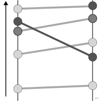
aussi : penteDeux axes reliés par des segments montrant le changement entre deux dates.
slopegraph
also: slope chartTwo axes joined by segments showing change between two points.
Classification
- graphique
- courbes et aires › courbes
- classement, évolution dans le temps; Visual Vocabulary du Financial Times
- le nom évoque : nature
Canaux
 position sur une échelle commune; principal : valeur aux deux dates
 inclinaison ou angle; principal : changement (pente du segment)
 teinte; secondaire : série
Attestation et synonymies
- terme français : Lagnel, Manuel de datavisualisation, Dunod, 2021
- définition anglaise : Visual Vocabulary du Financial Times
Littérature scientifique
OpenAlex : 47 articles depuis 1994, dont 32 % ces cinq dernières années; surtout en Computer Science, Engineering, Environmental Science
Références séminales
- invention (1983) Tufte (1983). The Visual Display of Quantitative Information. Graphics Press; Tufte 2001
Paquets R
- R
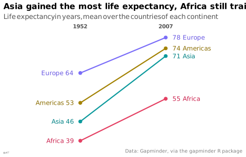
ggplot2::geom_line(); GitHub 7 025 étoiles; dernier commit 2026-10; article (33 455 citations) Une ligne par catégorie entre deux temps, avec geom_point aux extrémités.
Code R de l'exemple ggplot2
library(ggplot2)
library(dplyr)
library(gapminder)
## Oceania, two countries only, is left out.
life <- gapminder |>
filter(year %in% c(1952, 2007), continent != "Oceania") |>
group_by(continent, year) |>
summarise(lifeExp = mean(lifeExp), .groups = "drop")
start <- filter(life, year == 1952)
end <- filter(life, year == 2007)
## Names in the darker text colors of the continents, readable on white.
p <- ggplot(life, aes(x = factor(year), y = lifeExp, group = continent, colour = continent)) +
geom_line(linewidth = 0.8) +
geom_point(size = 2) +
geom_text(data = start, aes(label = paste(continent, round(lifeExp))),
colour = continent_text_colors[as.character(start$continent)],
hjust = 1, nudge_x = -0.08, size = 3.2) +
geom_text(data = end, aes(label = paste(round(lifeExp), continent)),
colour = continent_text_colors[as.character(end$continent)],
hjust = 0, nudge_x = 0.08, size = 3.2) +
scale_x_discrete(position = "top", expand = expansion(add = 0.9)) +
scale_y_continuous(NULL, breaks = NULL) +
scale_colour_manual(values = continent_colors) +
labs(title = "Asia gained the most life expectancy, Africa still trails",
subtitle = "Life expectancy in years, mean over the countries of each continent",
x = NULL,
caption = "Data: Gapminder, via the gapminder R package") +
theme_lex_viz(grid = "", arrows = "") +
theme(legend.position = "none", axis.text.x = element_text(face = "bold"))Sources (17)
115 occurrences dans le corpus; indexé par 8 ouvrages
Afficher les 17 sources
- Better data visualizations: a guide for scholars, researchers, and wonks
- Data visualisation: a handbook for data driven design
- Data visualization handbook
- Effective data storytelling: how to drive change with data, narrative, and visuals
- Effective data visualization: the right chart for the right data
- La graphique et le traitement graphique de l'information
- Lagnel, Manuel de datavisualisation, Dunod, 2021
- Les fondamentaux de la visualisation de données
- Manuel de datavisualisation - 2e éd, vol. 2
- Practical charts: the essential guide to creating clear, compelling charts for reports ...
- Semiologie graphique: les diagrammes, les réseaux, les cartes.
- Storytelling with data: let's practice!
- The big book of dashboards: visualizing your data using real-world business scenarios
- The functional art: an introduction to information graphics and visualization
- The Truthful Art: Data, Charts, and Maps for Communication
- Visual Vocabulary du Financial Times
- Wilke, Fundamentals of Data Visualization, O'Reilly, 2019
Citer cette fiche
Adresse stablehttps://dataviz.adrientaudiere.com/terme/slopegraph.html
RéférenceTaudière Adrien. 2026. graphique en pente. Dans Visualization Vocabulary, version 1.0.0. IdEst. https://dataviz.adrientaudiere.com/terme/slopegraph.html
BibTeX
@incollection{taudiere2026-slopegraph,
  author    = {Taudière, Adrien},
  title     = {graphique en pente},
  booktitle = {Visualization Vocabulary},
  year      = {2026},
  version   = {1.0.0},
  publisher = {IdEst},
  url       = {https://dataviz.adrientaudiere.com/terme/slopegraph.html},
  note      = {CC0 1.0}
}Fiche créée le 13/10/2026. Texte modifié le 12/11/2026. Images modifiées le 12/11/2026. Chiffres calculés le 22/10/2026.