
 chart
confection
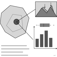
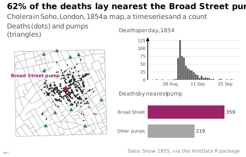
Assembly of visual events drawn from various sources and juxtaposed to carry an argument.
Classification
- chart
- non-chart figures
Attestation
- English definition: Tufte, Visual Explanations, 1997
Seminal references
- naming (1997) Tufte (1997). Visual Explanations: Images and Quantities, Evidence and Narrative. Graphics Press; Visual explanations: images and quantities
R code of the ggplot2 example
library(ggplot2)
library(dplyr)
library(HistData)
library(patchwork)
## Three pieces of different kinds, set side by side for one argument about
## the 1854 cholera outbreak in Soho: a map, a time series, a count.
nearest <- apply(Snow.deaths[, c("x", "y")], 1, function(d) {
Snow.pumps$label[which.min((Snow.pumps$x - d[1])^2 + (Snow.pumps$y - d[2])^2)]
})
by_pump <- tibble(pump = ifelse(nearest == "Broad St", "Broad Street", "Other pumps")) |>
count(pump) |>
mutate(pump = factor(pump, levels = c("Other pumps", "Broad Street")))
broad <- filter(Snow.pumps, label == "Broad St")
no_bg <- theme(plot.background = element_rect(fill = NA, colour = NA))
map <- ggplot() +
geom_path(data = Snow.streets, aes(x = x, y = y, group = street), colour = "#a6a6a6", linewidth = 0.3) +
geom_point(data = Snow.deaths, aes(x = x, y = y), colour = "#262626", size = 0.3) +
geom_point(data = Snow.pumps, aes(x = x, y = y), shape = 17, colour = "#2e7891", size = 1.8) +
geom_point(data = broad, aes(x = x, y = y), shape = 17, colour = "#9b2367", size = 2.8) +
annotate("label", x = broad$x - 0.8, y = broad$y + 2.4, label = "Broad Street pump",
colour = "#9b2367", fill = "white", linewidth = 0, size = 2.4, hjust = 1, fontface = "bold") +
coord_equal(xlim = c(3, 20), ylim = c(3, 20)) +
labs(subtitle = "Deaths (dots) and pumps (triangles)") +
theme_lex_viz(grid = "", arrows = "") +
theme(axis.text = element_blank(), axis.title = element_blank()) + no_bg
curve <- ggplot(filter(Snow.dates, !is.na(date)), aes(x = date, y = deaths)) +
geom_col(fill = "#535353", width = 0.8) +
scale_x_date(labels = scales::label_date("%d %b", locale = "en"), date_breaks = "2 weeks") +
scale_y_continuous(expand = expansion(mult = c(0, 0.05))) +
labs(subtitle = "Deaths per day, 1854", x = NULL, y = NULL) +
theme_lex_viz(base_size = 8, grid = "y", arrows = "y") + no_bg
pumps <- ggplot(by_pump, aes(x = n, y = pump, fill = pump)) +
geom_col(width = 0.7) +
geom_text(aes(label = n), hjust = -0.2, size = 2.4, colour = "#262626") +
scale_fill_manual(values = c(`Broad Street` = "#9b2367", `Other pumps` = "#a6a6a6"), guide = "none") +
scale_x_continuous(expand = expansion(mult = c(0, 0.2))) +
labs(subtitle = "Deaths by nearest pump", x = NULL, y = NULL) +
theme_lex_viz(base_size = 8, grid = "", arrows = "") +
theme(axis.text.x = element_blank()) + no_bg
p <- map + (curve / pumps) +
plot_layout(widths = c(1.15, 1)) +
plot_annotation(
title = "62% of the deaths lay nearest the Broad Street pump",
subtitle = "Cholera in Soho, London, 1854: a map, a time series and a count",
caption = "Data: Snow 1855, via the HistData R package",
theme = theme_lex_viz() + no_bg
) &
no_bgSources (5)
25 occurrences in the corpus; indexed by 1 book
Cite this entry
Stable addresshttps://dataviz.adrientaudiere.com/en-only/term/confection.html
ReferenceTaudière Adrien. 2026. confection. In Visualization Vocabulary, version 1.0.0. IdEst. https://dataviz.adrientaudiere.com/en-only/term/confection.html
BibTeX
@incollection{taudiere2026-confection,
  author    = {Taudière, Adrien},
  title     = {confection},
  booktitle = {Visualization Vocabulary},
  year      = {2026},
  version   = {1.0.0},
  publisher = {IdEst},
  url       = {https://dataviz.adrientaudiere.com/en-only/term/confection.html},
  note      = {CC0 1.0}
}Page created on 2026-10-13. Text last changed on 2026-11-02. Images last changed on 2026-11-12. Numbers computed on 2026-10-22.