
 graphique
confection
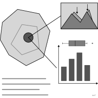
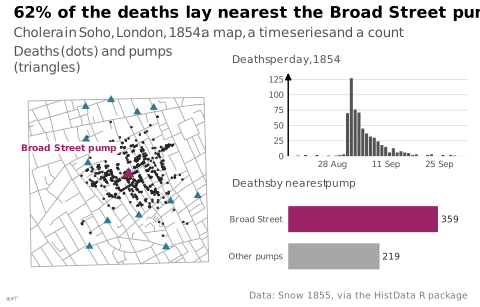
Assemblage d'images d'origines diverses juxtaposées pour porter un argument.
confection
Assembly of visual events drawn from various sources and juxtaposed to carry an argument.
Terme de Tufte, sans équivalent français établi. Ni carte ni graphique conventionnel : ce que le collage est à l'art, la confection l'est au design d'information.
Classification
- graphique
- hors graphique
Attestation
- terme français : Usage courant, non attesté par une source
- définition anglaise : Tufte, Visual Explanations, 1997
Références séminales
- nom (1997) Tufte (1997). Visual Explanations: Images and Quantities, Evidence and Narrative. Graphics Press; Visual explanations: images and quantities
Code R de l'exemple ggplot2
library(ggplot2)
library(dplyr)
library(HistData)
library(patchwork)
## Three pieces of different kinds, set side by side for one argument about
## the 1854 cholera outbreak in Soho: a map, a time series, a count.
nearest <- apply(Snow.deaths[, c("x", "y")], 1, function(d) {
Snow.pumps$label[which.min((Snow.pumps$x - d[1])^2 + (Snow.pumps$y - d[2])^2)]
})
by_pump <- tibble(pump = ifelse(nearest == "Broad St", "Broad Street", "Other pumps")) |>
count(pump) |>
mutate(pump = factor(pump, levels = c("Other pumps", "Broad Street")))
broad <- filter(Snow.pumps, label == "Broad St")
no_bg <- theme(plot.background = element_rect(fill = NA, colour = NA))
map <- ggplot() +
geom_path(data = Snow.streets, aes(x = x, y = y, group = street), colour = "#a6a6a6", linewidth = 0.3) +
geom_point(data = Snow.deaths, aes(x = x, y = y), colour = "#262626", size = 0.3) +
geom_point(data = Snow.pumps, aes(x = x, y = y), shape = 17, colour = "#2e7891", size = 1.8) +
geom_point(data = broad, aes(x = x, y = y), shape = 17, colour = "#9b2367", size = 2.8) +
annotate("label", x = broad$x - 0.8, y = broad$y + 2.4, label = "Broad Street pump",
colour = "#9b2367", fill = "white", linewidth = 0, size = 2.4, hjust = 1, fontface = "bold") +
coord_equal(xlim = c(3, 20), ylim = c(3, 20)) +
labs(subtitle = "Deaths (dots) and pumps (triangles)") +
theme_lex_viz(grid = "", arrows = "") +
theme(axis.text = element_blank(), axis.title = element_blank()) + no_bg
curve <- ggplot(filter(Snow.dates, !is.na(date)), aes(x = date, y = deaths)) +
geom_col(fill = "#535353", width = 0.8) +
scale_x_date(labels = scales::label_date("%d %b", locale = "en"), date_breaks = "2 weeks") +
scale_y_continuous(expand = expansion(mult = c(0, 0.05))) +
labs(subtitle = "Deaths per day, 1854", x = NULL, y = NULL) +
theme_lex_viz(base_size = 8, grid = "y", arrows = "y") + no_bg
pumps <- ggplot(by_pump, aes(x = n, y = pump, fill = pump)) +
geom_col(width = 0.7) +
geom_text(aes(label = n), hjust = -0.2, size = 2.4, colour = "#262626") +
scale_fill_manual(values = c(`Broad Street` = "#9b2367", `Other pumps` = "#a6a6a6"), guide = "none") +
scale_x_continuous(expand = expansion(mult = c(0, 0.2))) +
labs(subtitle = "Deaths by nearest pump", x = NULL, y = NULL) +
theme_lex_viz(base_size = 8, grid = "", arrows = "") +
theme(axis.text.x = element_blank()) + no_bg
p <- map + (curve / pumps) +
plot_layout(widths = c(1.15, 1)) +
plot_annotation(
title = "62% of the deaths lay nearest the Broad Street pump",
subtitle = "Cholera in Soho, London, 1854: a map, a time series and a count",
caption = "Data: Snow 1855, via the HistData R package",
theme = theme_lex_viz() + no_bg
) &
no_bgSources (7)
25 occurrences dans le corpus; indexé par 1 ouvrage
- Beautiful evidence
- Data visualization handbook
- Rakotomalala, fascicules de cours de statistique (Université Lyon 2)
- Seeing with fresh eyes: meaning, space, data, truth
- Semiologie graphique: les diagrammes, les réseaux, les cartes.
- Tufte, Visual Explanations, 1997
- Visual explanations: images and quantities, evidence and narrative
Citer cette fiche
Adresse stablehttps://dataviz.adrientaudiere.com/terme/confection.html
RéférenceTaudière Adrien. 2026. confection. Dans Visualization Vocabulary, version 1.0.0. IdEst. https://dataviz.adrientaudiere.com/terme/confection.html
BibTeX
@incollection{taudiere2026-confection,
  author    = {Taudière, Adrien},
  title     = {confection},
  booktitle = {Visualization Vocabulary},
  year      = {2026},
  version   = {1.0.0},
  publisher = {IdEst},
  url       = {https://dataviz.adrientaudiere.com/terme/confection.html},
  note      = {CC0 1.0}
}Fiche créée le 13/10/2026. Texte modifié le 02/11/2026. Images modifiées le 12/11/2026. Chiffres calculés le 22/10/2026.