
 chart
Ishikawa diagram
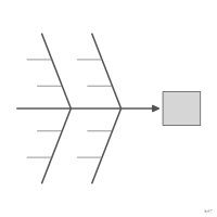
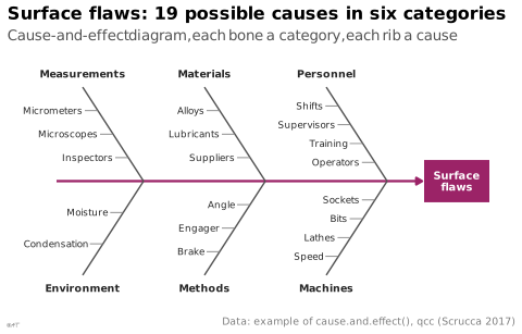
Fish-skeleton diagram that sorts the possible causes of an effect into categories, drawn as slanted bones along a central spine leading to the effect.
Classification
- chart
- networks and trees › hierarchical trees
- the name evokes: eponym
Channels
 tilt/angle; secondary: cause level (slanted bone for the category, horizontal for the cause)
 spatial region; main: cause category
Attestation and synonyms
- English definition: Information Graphics: A Comprehensive Illustrated Reference
- fishbone diagram; Information Graphics: A Comprehensive Illustrated Reference
- cause-and-effect diagram; Information Graphics: A Comprehensive Illustrated Reference
Scientific literature
OpenAlex: 9 441 papers since 1978, 51% in the last five years; mostly in Business, Management and Accounting, Engineering, Medicine; Wikidata
Seminal references
R packages
R code of the ggplot2 example
library(ggplot2)
library(dplyr)
## The example of qcc::cause.and.effect() (Scrucca 2017, GPL >= 2), copied
## here so that the script does not need qcc: the possible causes of surface
## flaws on machined parts, grouped by category. Categories above the spine,
## then below it, in the order of the help page.
causes <- list(
Measurements = c("Micrometers", "Microscopes", "Inspectors"),
Materials = c("Alloys", "Lubricants", "Suppliers"),
Personnel = c("Shifts", "Supervisors", "Training", "Operators"),
Environment = c("Condensation", "Moisture"),
Methods = c("Brake", "Engager", "Angle"),
Machines = c("Speed", "Lathes", "Bits", "Sockets")
)
dx <- 14 # horizontal run of a bone, from its outer end to the spine
bones <- tibble(category = names(causes), x = rep(c(6, 34, 62), 2),
y = rep(c(10, -10), each = 3)) |>
mutate(xend = x + dx, yend = 0)
## Each cause is a short horizontal rib on its bone, evenly spaced along it.
ribs <- bones |>
rowwise() |>
reframe(category = category, cause = causes[[category]],
t = seq_along(cause) / (length(cause) + 1),
xend = x + t * dx, y = y * (1 - t)) |>
mutate(x = xend - 3)
stopifnot(nrow(ribs) == 19, nrow(bones) == 6)
p <- ggplot() +
annotate("segment", x = 0, xend = 84, y = 0, yend = 0, colour = "#9b2367", linewidth = 0.8,
arrow = grid::arrow(length = unit(1.6, "mm"), type = "closed")) +
geom_segment(data = bones, aes(x = x, y = y, xend = xend, yend = yend), colour = "#535353", linewidth = 0.5) +
geom_segment(data = ribs, aes(x = x, y = y, xend = xend, yend = y), colour = "#7d7d7d", linewidth = 0.3) +
geom_text(data = ribs, aes(x = x - 0.5, y = y, label = cause), hjust = 1, size = 2.3, colour = "#262626") +
geom_text(data = bones, aes(x = x, y = y + 1.4 * sign(y), label = category),
fontface = "bold", size = 2.5, colour = "#262626") +
annotate("tile", x = 92, y = 0, width = 15, height = 4.5, fill = "#9b2367") +
annotate("text", x = 92, y = 0, label = "Surface\nflaws", colour = "white", fontface = "bold",
size = 2.6, lineheight = 0.9) +
scale_x_continuous(limits = c(-6, 100)) +
scale_y_continuous(limits = c(-12.5, 12.5)) +
labs(title = "Surface flaws: 19 possible causes in six categories",
subtitle = "Cause-and-effect diagram, each bone a category, each rib a cause",
x = NULL, y = NULL,
caption = "Data: example of cause.and.effect(), qcc (Scrucca 2017)") +
theme_lex_viz(grid = "", arrows = "") +
theme(axis.text = element_blank())Sources (2)
5 occurrences in the corpus
Cite this entry
Stable addresshttps://dataviz.adrientaudiere.com/en-only/term/ishikawa-diagram.html
ReferenceTaudière Adrien. 2026. Ishikawa diagram. In Visualization Vocabulary, version 1.0.0. IdEst. https://dataviz.adrientaudiere.com/en-only/term/ishikawa-diagram.html
BibTeX
@incollection{taudiere2026-ishikawa-diagram,
  author    = {Taudière, Adrien},
  title     = {Ishikawa diagram},
  booktitle = {Visualization Vocabulary},
  year      = {2026},
  version   = {1.0.0},
  publisher = {IdEst},
  url       = {https://dataviz.adrientaudiere.com/en-only/term/ishikawa-diagram.html},
  note      = {CC0 1.0}
}Page created on 2026-11-09. Text last changed on 2026-11-10. Images last changed on 2026-11-10. Numbers computed on 2026-10-22.