
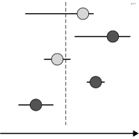
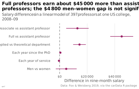
 chart
coefficient plot
also: dot-whisker plotModel coefficients and their intervals aligned on a common axis.
graphique des coefficients
aussi : graphique points-moustachesCoefficients d'un modèle et leurs intervalles alignés sur un axe commun.
Remplace avantageusement le tableau de régression dans un article.
Classification
- chart
- points and bubbles › dots and intervals
- magnitude
- the name evokes: nature
Channels
 position on common scale; main: estimate
 length; main: confidence interval
 spatial region; main: variable
Variants
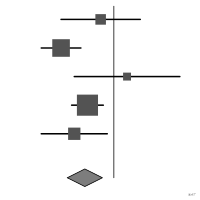 forest plotmeta-analysis
Attestation
- French term: Larmarange, guide-R: analysing survey data with R
Scientific literature
OpenAlex: 285 papers since 1975, 42% in the last five years; mostly in Engineering, Medicine, Chemistry
R packages
- R
dotwhisker::dwplot(); GitHub 59 stars; last commit 2026-06 - R
ggstats::ggcoef_model(); GitHub 56 stars; last commit 2026-09
R code of the ggplot2 example
library(ggplot2)
library(carData)
## Linear model of the 2008-09 nine-month salaries of US professors; each
## coefficient with its 95% interval, other variables held constant.
model <- lm(salary ~ rank + discipline + yrs.since.phd + yrs.service + sex, data = Salaries)
terms <- c(rankAssocProf = "Associate vs assistant professor", rankProf = "Full vs assistant professor",
disciplineB = "Applied vs theoretical department", yrs.since.phd = "Each year since the PhD",
yrs.service = "Each year of service", sexMale = "Men vs women")
coefs <- data.frame(term = terms[names(coef(model))[-1]], estimate = coef(model)[-1],
confint(model)[-1, ], check.names = FALSE)
names(coefs)[3:4] <- c("low", "high")
coefs$term <- factor(coefs$term, levels = rev(terms))
p <- ggplot(coefs, aes(x = estimate, y = term)) +
geom_vline(xintercept = 0, colour = "#535353", linewidth = 0.4, linetype = "dashed") +
geom_errorbar(aes(xmin = low, xmax = high), width = 0, orientation = "y", colour = "#9b2367",
linewidth = 0.6) +
geom_point(size = 2, colour = "#9b2367") +
scale_x_continuous(labels = \(x) paste0("$", lex_number(x))) +
labs(title = "Full professors earn about $45 000 more than assistant\nprofessors; the $4 800 men–women gap is not significant",
subtitle = "Salary differences in a linear model of 397 professors at one US college, 2008–09",
x = "Difference in nine-month salary", y = NULL,
caption = "Data: Fox & Weisberg 2019, via the carData R package") +
theme_lex_viz(grid = "x", arrows = "")Sources (3)
1 occurrence in the corpus
Cite this entry
Stable addresshttps://dataviz.adrientaudiere.com/en/term/coefficient-plot.html
ReferenceTaudière Adrien. 2026. coefficient plot. In Visualization Vocabulary, version 1.0.0. IdEst. https://dataviz.adrientaudiere.com/en/term/coefficient-plot.html
BibTeX
@incollection{taudiere2026-coefficient-plot,
  author    = {Taudière, Adrien},
  title     = {coefficient plot},
  booktitle = {Visualization Vocabulary},
  year      = {2026},
  version   = {1.0.0},
  publisher = {IdEst},
  url       = {https://dataviz.adrientaudiere.com/en/term/coefficient-plot.html},
  note      = {CC0 1.0}
}Page created on 2026-10-13. Text last changed on 2026-11-02. Images last changed on 2026-11-12. Numbers computed on 2026-10-22.