


 graphique
diagramme radar
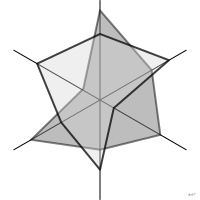
aussi : graphique en toile d'araignéeAxes rayonnants depuis un centre reliés par un polygone.
radar chart
also: spider chart, star plotAxes radiating from a center joined into a polygon.
Classification
- graphique
- radial › lignes polaires
- grandeur; Visual Vocabulary du Financial Times
- le nom évoque : nature, objet
Canaux
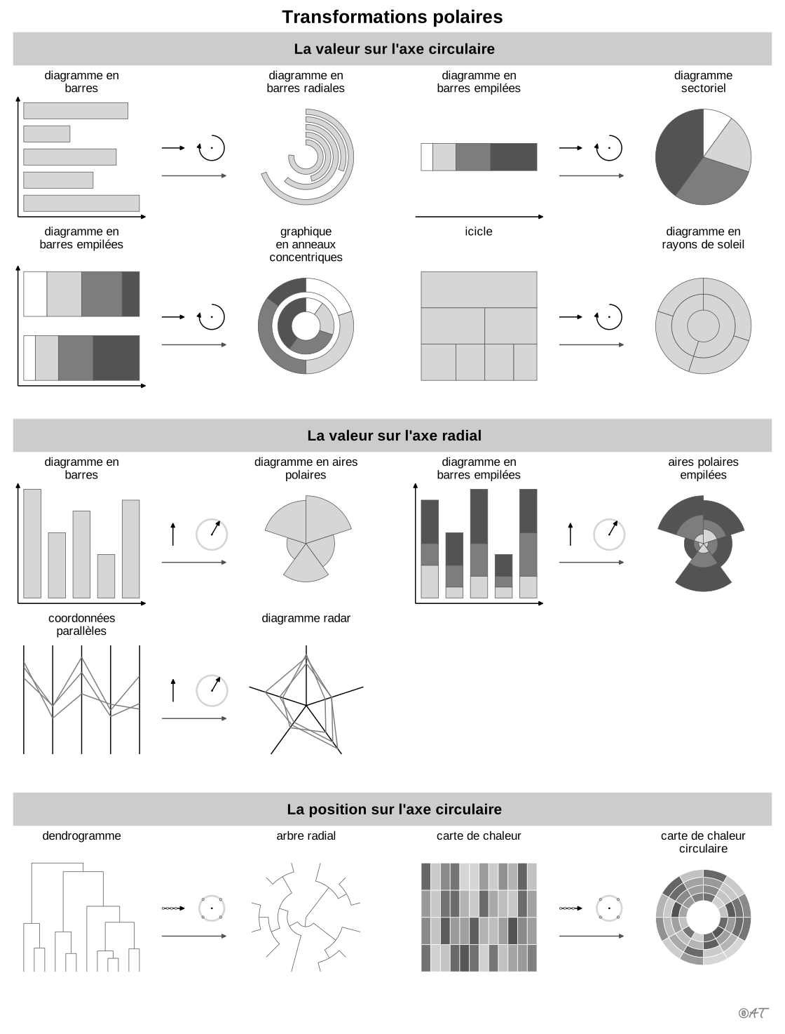
 position sur des échelles non alignées; principal : valeur sur chaque axe
 aire; secondaire : profil d'ensemble (surface du polygone, qui dépend de l'ordre des axes)
 région de l'espace; principal : variable (une direction par variable)
Attestation et synonymies
- terme français : Lagnel, Manuel de datavisualisation, Dunod, 2021
- définition anglaise : Data Visualisation Guide, data.europa.eu
- diagramme de Kiviat; Wikipédia en français↗
Littérature scientifique
OpenAlex : 2 490 articles depuis 1956, dont 56 % ces cinq dernières années; surtout en Engineering, Computer Science, Social Sciences; Wikidata
Références séminales
- premier usage connu (1877) von Mayr (1877). Die Gesetzmässigkeit im Gesellschaftsleben; Ciuccarelli 2026, Friendly & Denis 2001
Code R de l'exemple ggplot2
library(ggplot2)
library(dplyr)
library(tidyr)
library(palmerpenguins)
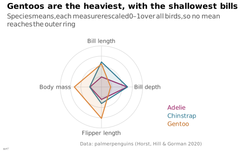
## Each measure rescaled from 0 to 1 over all the birds, then averaged by
## species: the spokes compare species without stretching their differences.
measures <- c(bill_length_mm = "Bill length", bill_depth_mm = "Bill depth",
flipper_length_mm = "Flipper length", body_mass_g = "Body mass")
means <- penguins |>
pivot_longer(all_of(names(measures)), names_to = "measure", values_to = "value") |>
filter(!is.na(value)) |>
group_by(measure) |>
mutate(value = (value - min(value)) / (max(value) - min(value))) |>
group_by(species, measure) |>
summarise(value = mean(value), .groups = "drop")
## Polygons drawn in plain x-y coordinates: one spoke per measure, clockwise from the top.
angle <- setNames(pi / 2 - 2 * pi * (seq_along(measures) - 1) / length(measures), names(measures))
polygons <- means |>
mutate(x = value * cos(angle[measure]), y = value * sin(angle[measure]))
rings <- expand_grid(r = c(0.25, 0.5, 0.75, 1), t = seq(0, 2 * pi, length.out = 121)) |>
mutate(x = r * cos(t), y = r * sin(t))
spokes <- tibble(measure = measures, x = cos(angle), y = sin(angle))
p <- ggplot(polygons, aes(x = x, y = y)) +
geom_path(data = rings, aes(group = r), colour = "#d6d6d6", linewidth = 0.3) +
geom_segment(data = spokes, aes(x = 0, y = 0, xend = x, yend = y), colour = "#d6d6d6", linewidth = 0.3) +
geom_text(data = spokes, aes(x = 1.12 * x, y = 1.12 * y, label = measure), size = 3, colour = "#535353") +
geom_polygon(aes(colour = species, fill = species), alpha = 0.12, linewidth = 0.7) +
annotate("text", x = c(1.6, 1.6, 1.6), y = c(-0.5, -0.7, -0.9),
label = c("Adelie", "Chinstrap", "Gentoo"), colour = c("#9b2367", "#2e7891", "#c06a1f"),
hjust = 0, size = 3.2) +
coord_fixed(xlim = c(-1.35, 2.25), ylim = c(-1.15, 1.15)) +
labs(title = "Gentoos are the heaviest, with the shallowest bills",
subtitle = "Species means, each measure rescaled 0–1 over all birds, so no mean reaches the outer ring",
x = NULL, y = NULL,
caption = "Data: palmerpenguins (Horst, Hill & Gorman 2020)") +
theme_lex_viz(grid = "", arrows = "") +
theme(legend.position = "none", axis.text = element_blank())Sources (27)
108 occurrences dans le corpus; indexé par 11 ouvrages
Afficher les 27 sources
- app.flourish.studio
- Atlas of knowledge: anyone can map
- Better data visualizations: a guide for scholars, researchers, and wonks
- Data points: visualization that means something
- Data Visualisation Guide, data.europa.eu
- Data visualisation: a handbook for data driven design
- data-to-viz.com
- Effective data storytelling: how to drive change with data, narrative, and visuals
- Exploratory Data Analysis: Descriptive Analysis, Visualization, and Dashboard Design (w...
- From data to viz
- Interactive data visualization: foundations, techniques, and applications
- Lagnel, Manuel de datavisualisation, Dunod, 2021
- Les fondamentaux de la visualisation de données
- Manuel de datavisualisation - 2e éd, vol. 2
- Milestones in the history of thematic cartography, statistical graphics, and data visua...
- Questions in Dataviz: A Design-Driven Process for Data Visualisation
- Show me the numbers: designing tables and graphs to enlighten
- The book of circles: visualizing spheres of knowledge
- The functional art: an introduction to information graphics and visualization
- The grammar of graphics
- The Truthful Art: Data, Charts, and Maps for Communication
- The Wall Street journal guide to information graphics: the dos and don'ts of presenting...
- Thematic Cartography and Geovisualization
- Visual strategies for biological data
- Visualization of Time-Oriented Data
- Wikipedia — Data and information visualization
- Wikipedia in English↗
Citer cette fiche
Adresse stablehttps://dataviz.adrientaudiere.com/terme/radar-chart.html
RéférenceTaudière Adrien. 2026. diagramme radar. Dans Visualization Vocabulary, version 1.0.0. IdEst. https://dataviz.adrientaudiere.com/terme/radar-chart.html
BibTeX
@incollection{taudiere2026-radar-chart,
  author    = {Taudière, Adrien},
  title     = {diagramme radar},
  booktitle = {Visualization Vocabulary},
  year      = {2026},
  version   = {1.0.0},
  publisher = {IdEst},
  url       = {https://dataviz.adrientaudiere.com/terme/radar-chart.html},
  note      = {CC0 1.0}
}Fiche créée le 13/10/2026. Texte modifié le 06/11/2026. Images modifiées le 12/11/2026. Chiffres calculés le 22/10/2026.