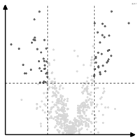
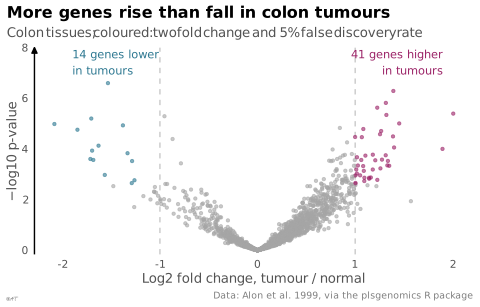
graphique en volcan

Code R de l'exemple ggplot2

library(ggplot2)
library(plsgenomics)

## 2 000 genes in 40 colon tumours and 22 normal tissues: log2 fold change of
## the means and Welch t-test, p-values adjusted by Benjamini-Hochberg.
data(Colon)
expression <- log2(Colon$X)
tumour <- Colon$Y == 2
genes <- data.frame(
  change = colMeans(expression[tumour, ]) - colMeans(expression[!tumour, ]),
  p = apply(expression, 2, \(g) t.test(g[tumour], g[!tumour])$p.value)
)
genes$q <- p.adjust(genes$p, method = "BH")
genes$group <- with(genes, ifelse(q < 0.05 & change > 1, "Higher in tumours",
                           ifelse(q < 0.05 & change < -1, "Lower in tumours", "Other")))
counts <- table(genes$group)

p <- ggplot(genes, aes(x = change, y = -log10(p), colour = group)) +
  geom_vline(xintercept = c(-1, 1), colour = "#a6a6a6", linewidth = 0.3, linetype = "dashed") +
  geom_point(size = 0.9, alpha = 0.6) +
  annotate("text", x = c(1.9, -1.9), y = 7.9, hjust = c(1, 0), vjust = 1, size = 3, colour = c("#9b2367", "#2e7891"),
           label = paste(counts[c("Higher in tumours", "Lower in tumours")],
                         c("genes higher\nin tumours", "genes lower\nin tumours"))) +
  scale_colour_manual(values = c(`Higher in tumours` = "#9b2367", `Lower in tumours` = "#2e7891",
                                 Other = "#a6a6a6")) +
  scale_x_continuous(labels = lex_number) +
  scale_y_continuous(labels = lex_number, limits = c(0, 8), expand = expansion(mult = c(0.02, 0))) +
  labs(title = "More genes rise than fall in colon tumours",
       subtitle = "Colon tissues; coloured: twofold change and 5% false discovery rate",
       x = "Log2 fold change, tumour / normal", y = "−log10 p-value",
       caption = "Data: Alon et al. 1999, via the plsgenomics R package") +
  theme_lex_viz(grid = "", arrows = "y") +
  theme(legend.position = "none")