
 graphique
diagramme alluvial
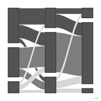
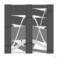
Blocs empilés à chaque étape d'une suite ordonnée, reliés d'une étape à la suivante par des bandes dont l'épaisseur code l'effectif qui passe d'un groupe à l'autre.
alluvial diagram
Blocks stacked at each stage of an ordered sequence, linked from one stage to the next by bands whose width encodes the count moving from one group to another.
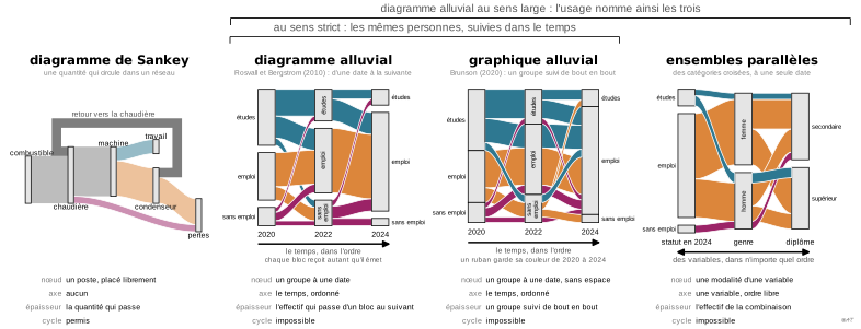
Introduit par Rosvall et Bergstrom (2010) pour le changement de structure d'un réseau : les blocs y sont espacés et chaque bande ne relie que deux étapes voisines, si bien qu'un bloc reçoit autant qu'il émet. Au sens large, le terme inclut les ensembles parallèles et le graphique alluvial de Brunson (2020), qui suit un même groupe de bout en bout. Plusieurs sources en font une forme du diagramme de Sankey.
Classification
- graphique
- flux › flux en rubans
- flux, évolution dans le temps
- le nom évoque : nature
Canaux
 longueur; principal : effectif de chaque groupe et de chaque flux
 aire; secondaire : effectif de chaque groupe et de chaque flux
 région de l'espace; principal : date et groupe
 teinte; secondaire : groupe de départ du flux
Variantes
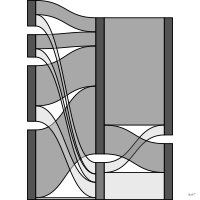 ensembles parallèlesvariables qualitatives sans ordre
 graphique alluvialrubans de bout en bout
Attestation et synonymies
- terme français : Larmarange, guide-R : guide pour l'analyse de données d'enquêtes avec R
- définition anglaise : Rosvall & Bergstrom, Mapping Change in Large Networks, PLoS ONE, 2010↗
- alluvial graph; Atlas of knowledge: anyone can map
Références séminales
- nom (2010) Rosvall & Bergstrom (2010). Mapping change in large networks. PLoS ONE (650 citations); Ciuccarelli 2026
Paquets R
- R
ggalluvial::geom_flow(); GitHub 526 étoiles; dernier commit 2026-02; article (536 citations) - R
alluvial::alluvial(); GitHub 147 étoiles; dernier commit 2026-05; article (33 citations)
Code R de l'exemple ggplot2
library(ggplot2)
library(dplyr)
library(tidyr)
library(ggalluvial)
library(gapminder)
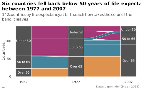
## Countries by life-expectancy band in 1952, 1977 and 2007. As in Rosvall &
## Bergstrom (2010), flows only join adjacent dates (geom_flow): each flow
## takes the color of the band it leaves, and a band receives as much as it
## sends.
bands <- gapminder |>
filter(year %in% c(1952, 1977, 2007)) |>
mutate(band = cut(lifeExp, c(0, 50, 65, Inf), right = FALSE,
labels = c("Under 50", "50 to 65", "Over 65"))) |>
select(country, year, band)
p <- ggplot(bands, aes(x = factor(year), stratum = band, alluvium = country)) +
geom_flow(aes(fill = band), aes.flow = "forward", width = 0.3, colour = "white",
linewidth = 0.2, alpha = 0.9) +
geom_stratum(width = 0.3, fill = "#535353", colour = "white", linewidth = 0.3) +
geom_text(stat = "stratum", aes(label = after_stat(stratum)), colour = "white", size = 2.8) +
scale_fill_manual(values = unname(lex_colors)) +
scale_x_discrete(expand = expansion(add = 0.2)) +
labs(title = "Six countries fell back below 50 years of life expectancy\nbetween 1977 and 2007",
subtitle = "142 countries by life expectancy at birth; each flow takes the color\nof the band it leaves",
x = NULL, y = "Countries",
caption = "Data: gapminder (Bryan 2025)") +
theme_lex_viz(grid = "", arrows = "") +
theme(legend.position = "none", axis.text.x = element_text(face = "bold"))Sources (8)
36 occurrences dans le corpus; indexé par 1 ouvrage
- Bremer & Barone, Chart, CRC Press, 2025
- Data visualisation: a handbook for data driven design
- Design for information: an introduction to the histories, theories, and best practices ...
- Larmarange, guide-R : guide pour l'analyse de données d'enquêtes avec R
- Rosvall & Bergstrom, Mapping Change in Large Networks, PLoS ONE, 2010↗
- The art of insight: how great visualization designers think
- Visualization of Time-Oriented Data
- Visualize This
Citer cette fiche
Adresse stablehttps://dataviz.adrientaudiere.com/terme/alluvial-diagram.html
RéférenceTaudière Adrien. 2026. diagramme alluvial. Dans Visualization Vocabulary, version 1.0.0. IdEst. https://dataviz.adrientaudiere.com/terme/alluvial-diagram.html
BibTeX
@incollection{taudiere2026-alluvial-diagram,
  author    = {Taudière, Adrien},
  title     = {diagramme alluvial},
  booktitle = {Visualization Vocabulary},
  year      = {2026},
  version   = {1.0.0},
  publisher = {IdEst},
  url       = {https://dataviz.adrientaudiere.com/terme/alluvial-diagram.html},
  note      = {CC0 1.0}
}Fiche créée le 10/11/2026. Texte modifié le 12/11/2026. Images modifiées le 11/11/2026. Chiffres calculés le 22/10/2026.