
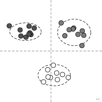
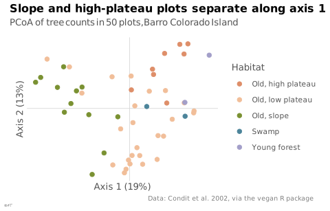
 graphique
ordination
Projection d'objets décrits par de nombreuses variables dans un espace de faible dimension.
ordination
Projection of objects described by many variables into a low-dimensional space.
Terme d'écologie numérique : ACP, AFC, NMDS et PCoA en sont des cas.
Classification
- graphique
- points et bulles › nuages de points
- corrélation
Canaux
 position sur une échelle commune; principal : coordonnées sur les axes
 teinte; secondaire : groupe
 forme; secondaire : groupe
Variantes
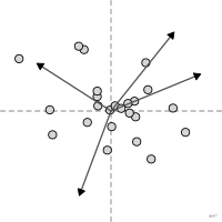 biplotvariables en flèches
Attestation
- terme français : Wikipédia en français
Littérature scientifique
OpenAlex : 578 articles depuis 1977, dont 18 % ces cinq dernières années; surtout en Environmental Science, Agricultural and Biological Sciences, Earth and Planetary Sciences; Wikidata
Références séminales
- premier usage connu (1901) Pearson (1901). On lines and planes of closest fit to systems of points in space. The London, Edinburgh, and Dublin Philosophical Magazine and Journal of Science (12 781 citations); Wikipedia in English
Paquets R
- R
vegan::ordiplot(); GitHub 551 étoiles; dernier commit 2026-10 - R
barrel::stat_barrel(); article (0 citations)
Code R de l'exemple ggplot2
library(ggplot2)
library(vegan)
## Principal coordinates of the Bray-Curtis dissimilarities between plots.
data(BCI, BCI.env)
pcoa <- cmdscale(vegdist(BCI, method = "bray"), k = 2, eig = TRUE)
share <- scales::percent(pcoa$eig[1:2] / sum(pcoa$eig[pcoa$eig > 0]), accuracy = 1)
habitats <- c(OldHigh = "Old, high plateau", OldLow = "Old, low plateau", OldSlope = "Old, slope",
Swamp = "Swamp", Young = "Young forest")
plots <- data.frame(pcoa$points, habitat = habitats[as.character(BCI.env$Habitat)])
p <- ggplot(plots, aes(x = X1, y = X2, colour = habitat)) +
geom_hline(yintercept = 0, colour = "#d6d6d6", linewidth = 0.3) +
geom_vline(xintercept = 0, colour = "#d6d6d6", linewidth = 0.3) +
geom_point(size = 2) +
coord_fixed() +
labs(title = "Slope and high-plateau plots separate along axis 1",
subtitle = "PCoA of tree counts in 50 plots, Barro Colorado Island",
x = paste0("Axis 1 (", share[1], ")"), y = paste0("Axis 2 (", share[2], ")"),
colour = "Habitat",
caption = "Data: Condit et al. 2002, via the vegan R package") +
theme_lex_viz(grid = "", arrows = "") +
theme(axis.text = element_blank(), legend.position = "right", legend.direction = "vertical")Sources (9)
366 occurrences dans le corpus
- Applied Multivariate Statistics in R
- Cartographies of Time
- Fiches de biostatistique du PBIL (Chessel, Dufour, Thioulouse et al., Lyon 1)
- Grosjean & Engels, Science des données biologiques I-III (Université de Mons)
- Série d'ateliers R du CSBQ, version française (Centre de la science de la biodiversité du Québec)
- Visualization Analysis and Design
- Wikipedia — Data and information visualization
- Wikipédia en français
- Wikipedia in English↗ fr
Citer cette fiche
Adresse stablehttps://dataviz.adrientaudiere.com/terme/ordination.html
RéférenceTaudière Adrien. 2026. ordination. Dans Visualization Vocabulary, version 1.0.0. IdEst. https://dataviz.adrientaudiere.com/terme/ordination.html
BibTeX
@incollection{taudiere2026-ordination,
  author    = {Taudière, Adrien},
  title     = {ordination},
  booktitle = {Visualization Vocabulary},
  year      = {2026},
  version   = {1.0.0},
  publisher = {IdEst},
  url       = {https://dataviz.adrientaudiere.com/terme/ordination.html},
  note      = {CC0 1.0}
}Fiche créée le 13/10/2026. Texte modifié le 02/11/2026. Images modifiées le 12/11/2026. Chiffres calculés le 22/10/2026.