

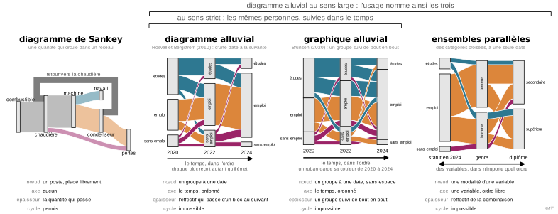

 graphique
diagramme de Sankey
Flux dont l'épaisseur code une quantité conservée entre étapes.
Sankey diagram
Flows whose width encodes a quantity conserved between stages.
Classification
- graphique
- flux › flux en rubans
- flux; Visual Vocabulary du Financial Times
- le nom évoque : nom de personne
Canaux
 longueur; principal : volume du flux (épaisseur du ruban)
 aire; secondaire : effectif de chaque modalité et de chaque flux
 région de l'espace; principal : étape et nœud
 teinte; secondaire : origine du flux
Variantes
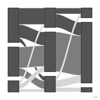 diagramme alluvialétapes ordonnées en colonnes
Attestation
- terme français : Lagnel, Manuel de datavisualisation, Dunod, 2021
- définition anglaise : Data Visualisation Guide, data.europa.eu
Littérature scientifique
OpenAlex : 1 824 articles depuis 1990, dont 69 % ces cinq dernières années; surtout en Medicine, Environmental Science, Computer Science; Wikidata
Références séminales
- premier usage connu (1869) Minard (1869). Carte figurative des pertes successives en hommes de l'armée française dans la campagne de Russie 1812-1813; Ciuccarelli 2026
- nom (1898) Kennedy & Sankey (1898). The thermal efficiency of steam engines: report of the committee. Minutes of the Proceedings of the Institution of Civil Engineers (69 citations); Andrews 2017, Ciuccarelli 2026
Paquets R
Code R de l'exemple ggplot2
library(ggplot2)
library(dplyr)
library(ggsankey) # on GitHub only: pak::pak("davidsjoberg/ggsankey")
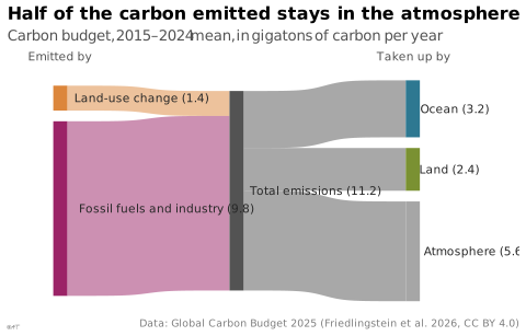
## The global carbon budget, mean of 2015-2024 (GtC per year), from the
## Global Carbon Budget 2025: what is emitted, then where it goes. Fossil
## emissions include the cement carbonation sink; the budget imbalance,
## under 0.1 GtC, is left out.
sources <- c(`Fossil fuels and industry` = 9.8, `Land-use change` = 1.4)
sinks <- c(Atmosphere = 5.6, Ocean = 3.2, Land = 2.4)
## One row per tenth of a gigatonne: the quantity is conserved from one
## stage to the next, and every row passes through the total.
carbon <- tibble(source = rep(names(sources), round(10 * sources)),
total = "Total emissions",
sink = rep(names(sinks), round(10 * sinks)))
values <- c(sources, `Total emissions` = sum(sources), sinks)
flows <- make_long(carbon, source, total, sink) |>
mutate(label = paste0(node, " (", sprintf("%.1f", values[node]), ")"))
p <- ggplot(flows, aes(x = x, next_x = next_x, node = node, next_node = next_node,
fill = node, label = label)) +
geom_sankey(flow.alpha = 0.5, node.color = NA, width = 0.08, space = 6) +
geom_sankey_text(hjust = -0.12, space = 6, size = 2.8, colour = "#262626") +
scale_fill_manual(values = c(`Fossil fuels and industry` = "#9b2367", `Land-use change` = "#dc863b",
`Total emissions` = "#535353", Atmosphere = "#a6a6a6",
Ocean = "#2e7891", Land = "#7a9132")) +
scale_x_discrete(labels = c(source = "Emitted by", total = "", sink = "Taken up by"),
position = "top", expand = expansion(add = c(0.3, 0.6))) +
labs(title = "Half of the carbon emitted stays in the atmosphere",
subtitle = "Carbon budget, 2015–2024 mean, in gigatons of carbon per year",
x = NULL, y = NULL,
caption = "Data: Global Carbon Budget 2025 (Friedlingstein et al. 2026, CC BY 4.0)") +
theme_lex_viz(grid = "", arrows = "") +
theme(legend.position = "none", axis.text.y = element_blank())Sources (28)
60 occurrences dans le corpus; indexé par 8 ouvrages
Afficher les 28 sources
- app.flourish.studio
- Atlas of knowledge: anyone can map
- Better data visualizations: a guide for scholars, researchers, and wonks
- Bremer & Barone, Chart, CRC Press, 2025
- Data Visualisation Guide, data.europa.eu
- Data visualisation: a handbook for data driven design
- Data visualization handbook
- Data Viz Project
- data-to-viz.com
- dataphys.org
- datavizcatalogue.com
- datavizproject.com
- datawrapper.de↗
- Design for information: an introduction to the histories, theories, and best practices ...
- Effective data storytelling: how to drive change with data, narrative, and visuals
- Effective data visualization: the right chart for the right data
- Exploratory Data Analysis: Descriptive Analysis, Visualization, and Dashboard Design (w...
- From data to viz
- Lagnel, Manuel de datavisualisation, Dunod, 2021
- Larmarange et al., analyse-R : introduction à l'analyse d'enquêtes avec R
- Larmarange, guide-R : guide pour l'analyse de données d'enquêtes avec R
- Open Visualization Academy, cours et lettre d'information (Cairo et al.)
- The Truthful Art: Data, Charts, and Maps for Communication
- Thematic Cartography and Geovisualization
- Visualization of Time-Oriented Data
- Wikipedia — Data and information visualization
- Wikipédia en français↗
- Wikipedia in English↗
Citer cette fiche
Adresse stablehttps://dataviz.adrientaudiere.com/terme/sankey-diagram.html
RéférenceTaudière Adrien. 2026. diagramme de Sankey. Dans Visualization Vocabulary, version 1.0.0. IdEst. https://dataviz.adrientaudiere.com/terme/sankey-diagram.html
BibTeX
@incollection{taudiere2026-sankey-diagram,
  author    = {Taudière, Adrien},
  title     = {diagramme de Sankey},
  booktitle = {Visualization Vocabulary},
  year      = {2026},
  version   = {1.0.0},
  publisher = {IdEst},
  url       = {https://dataviz.adrientaudiere.com/terme/sankey-diagram.html},
  note      = {CC0 1.0}
}Fiche créée le 13/10/2026. Texte modifié le 12/11/2026. Images modifiées le 12/11/2026. Chiffres calculés le 22/10/2026.